Appendix C — Intraclass Correlation

This annex quantifies baseline Intraclass Correlation Coefficient (ICC)-style diagnostics for Penta-1 coverage at the household, cluster, ward, and Local Government Area (LGA) levels. It uses the baseline multistage cluster survey (gold standard) as the empirical reference for design planning.¹

In survey operations, ICC matters because clustering inflates variance relative to simple random sampling (Kish 1965; Heeringa, West, and Berglund 2017). Values of ICC near 0 indicate weak within-group similarity at that level, while larger values indicate stronger local dependence. Knowing plausible ICC values helps set sample sizes to reach target precision. For planning, these estimates can replace default values for Design Effect (DEFF) with context-specific DEFF calculations based on the empirical ICC. When researchers control how many households to interview per cluster, increasing households per cluster usually increases DEFF when within-cluster correlation is positive, while reducing households per cluster and adding clusters usually improves precision at a fixed total sample size. That precision gain is not free: adding clusters increases travel, listing, supervision, and other field costs. These ICC-style diagnostics therefore support scenario-based budgeting to choose a households-per-cluster value that balances precision targets against operational cost constraints.

The term ICC has multiple definitions, so this annex states its definition explicitly before presenting results. For single-stage cluster designs, those definitions are often easier to reconcile because both reduce to a within-cluster correlation or equivalent variance-share parameter (Gelman and Hill 2006; Heeringa, West, and Berglund 2017). In multilevel modeling, level-specific ICC values are treated as additive variance shares from one nested random-effects model with a common variance denominator. In design-based survey practice, ICC is typically interpreted as the expected within-cluster correlation for a given sampling design (Lovasi et al. 2017). Even within the design-based survey community, most sampling-theory treatments and common complex-survey software routines use ICC in this single-stage sense. With two-stage and three-stage designs, differences become more apparent because dependence accumulates across nested levels and can be expressed either as decomposed level-specific components or as cumulative within-group correlation patterns (Chen and Rust 2017).

For each grouping variable, we compute a weighted variance-share statistic separately: \[ \rho_g^* = \frac{B_g}{B_g + W_g}, \tag{C.1}\]

where \(B_g\) is the weighted between-group sum of squares and \(W_g\) is the weighted within-group sum of squares for grouping variable \(g\). We then recompute \(\rho_g^*\) across generalized-bootstrap replicate weights to obtain a replicate distribution, a replicate-mean point estimate, and percentile uncertainty intervals. Because each level is estimated in a separate one-way decomposition, lower-level estimates are cumulative with respect to higher-level dependence. For example, the cluster-level ICC includes dependence shared through ward and LGA, and the ward-level ICC includes LGA-level dependence. These values are therefore not expected to sum to 1 across levels.

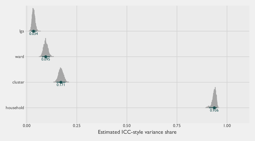
Figure Figure C.1 shows the replicate distributions for each level, and Table Table C.1 reports the corresponding replicate means and percentile intervals. The dominant result is the household estimate (0.936), which is much larger than the cluster (0.171), ward (0.095), and LGA (0.034) estimates. That pattern is consistent with strong within-household concordance in vaccination status and with the estimator property that households with one sampled child contribute no within-household sum of squares. Comparable large-scale survey analyses also find meaningful household and local-area clustering for immunization outcomes (Dwivedi et al. 2023). For design, this means that adding children within the same household usually contributes less independent information than adding households.

Under a simplified single-stage planning assumption, consistent with the ultimate-cluster variance approximation used in many survey software implementations, the usual formula is \(\textrm{DEFF} \approx 1 + (m - 1)\rho\) with cluster size \(m\). This approximation treats the sampled cluster as the primary unit of correlation and does not separately model lower-level nesting within clusters. If we use only the empirical cluster-level estimate from this annex and assume \(m = 7\) children per cluster, then the implied DEFF is approximately 2.02. This example is deliberately simplified and is intended only to show how an empirical ICC can be mapped into a working DEFF assumption.

Figure C.1: Replicate distribution of baseline ICC-style estimates by grouping level

Table Table C.1 presents the same results in compact numeric form for planning use.

Table C.1: Baseline Penta-1 ICC-style variance-share summary by grouping level

Level	Mean ICC	95% lower	95% upper
Household	0.936	0.910	0.950
Cluster	0.171	0.149	0.193
Ward	0.095	0.076	0.116
LGA	0.034	0.021	0.048

These diagnostics are descriptive design inputs rather than a standalone model of data-generating structure. The uncertainty intervals come from the generalized-bootstrap replicate design already used in the baseline pipeline. For each replicate weight vector, we recompute the ICC statistic at each level using the same weighted between-group and within-group decomposition. This yields the empirical replicate distributions in Figure C.1. The point estimates in Table C.1 are replicate means, and lower and upper limits represent a 95% bootstrap confidence interval. This bootstrap approach propagates complex-survey design uncertainty into the ICC diagnostics without requiring normal-approximation assumptions for the ICC statistic.

C.1 Stratum-Specific ICC

The pooled ICC estimates in Table C.1 combine data from both sentinel and non-sentinel strata. Because these strata used different first-stage sampling strategies, their clustering properties may differ in ways that matter for survey planning.

In the sentinel LGAs (Gabasawa, Gaya, Nassarawa), the gold-standard survey drew a direct stratified sample of building footprints rather than a first-stage cluster sample of enumeration areas, achieving broad spatial coverage within each LGA. By contrast, the non-sentinel stratum used a probability-proportional-to-size (Probability Proportional-to-Size (PPS)) first-stage selection of gridded enumeration areas, which is closer to the design a typical Expanded Programme on Immunization (EPI)-style survey would follow. To ensure an apples-to-apples comparison, Table C.2 uses the same gridded enumeration area unit as the cluster-level grouping in both strata, rather than the operational workload clusters used for field logistics in sentinel areas. The non-sentinel gridded-EA ICC is a more appropriate empirical reference for planning a conventional survey design such as the EPI 30 \(\times\) 7 benchmark, because it reflects the between-cluster variance encountered under genuine first-stage probability sampling.

Table C.2 presents the ICC estimates separately for sentinel and non-sentinel strata at the household, gridded enumeration area, and ward levels.

Table C.2: Baseline Penta-1 ICC by stratum type and grouping level

Stratum	Level	Mean ICC	95% lower	95% upper
Non-sentinel	Household	0.941	0.909	0.957
	Gridded EA	0.152	0.126	0.178
	Ward	0.104	0.082	0.128
Sentinel	Household	0.914	0.905	0.922
	Gridded EA	0.315	0.301	0.329
	Ward	0.037	0.030	0.045

C.2 Cost-Optimal Cluster Size

The ICC estimates above describe the statistical cost of within-cluster homogeneity. Pairing them with the operational cost structure recovered from the time-motion study yields an empirical estimate of the cost-optimal number of child interviews to conduct per cluster. Throughout this section \(m\) refers to the number of children 0–23 mo interviewed per cluster, which is the unit at which the empirical ICC is estimated and at which the per-interview cost denominator from this study’s cost decomposition is defined. The classic EPI \(30 \times 7\) benchmark is also specified in children (7 children aged 12–23 mo per cluster), so both quantities are on the same scale.

Kish (1965) showed that, for a single-stage cluster design with linear cost structure \[C = c_1 a + c_2 a m, \tag{C.2}\] where \(a\) is the number of clusters and \(m\) is the number of within-cluster interviews (here, children 0–23 mo), the cluster size that minimizes total cost at a fixed effective sample size (or equivalently, maximizes effective sample size at fixed cost) is \[m_{\text{opt}} = \sqrt{\frac{c_1\,(1-\rho)}{c_2\,\rho}}, \tag{C.3}\] where \(c_1\) is the cost of adding a new cluster (transport, listing, supervision), \(c_2\) is the cost of interviewing one additional child within an existing cluster, and \(\rho\) is the cluster-level ICC of the outcome. The expression is symmetric in \(\rho\) and the cost ratio: large \(\rho\) (high within-cluster homogeneity) pushes \(m_{\text{opt}}\) down, while a large \(c_1/c_2\) (cluster overhead dominates per-interview cost) pushes \(m_{\text{opt}}\) up (Kish 1965; Heeringa, West, and Berglund 2017).

We estimate \(c_1/c_2\) in two ways to bracket the structural uncertainty in how field costs decompose between cluster overhead and within-cluster interview effort.

Decomposition A (time-weighted, all costs). We split the observed per-cluster field cost from Table 4.21 by the time fraction spent on non-interview work. From the time-motion event log, the median enumerator-day breaks down into roughly 204 minutes of overhead (assembly, travel, return) and 420 minutes of fieldwork inside the enumeration area, so the overhead share of the field day is approximately 33%.² Applied to the Gold-Standard core (Conventional + Network Scale-Up Method (NSUM)) marginal cost of $113.69 per cluster and 11.3 children per cluster, this gives \(c_1 \approx\) $37.18 and \(c_2 \approx\) $6.77, a ratio of \(c_1/c_2 \approx\) 5.5. Under this decomposition, every dollar of daily cost is treated as proportional to where the day’s minutes are spent. This time-weighting is a planning-grade allocation of total observed cost, not a strict cost elasticity in \(m\): in particular, supervisor labour is paid as a daily rate rather than per interview, so its share is partly cluster-fixed. Decomposition B addresses this directly.

Decomposition B (supervisor as cluster-fixed). The supervisor day rate ($70) is paid once per team-day and includes vehicle and fuel, so adding interviews to an existing cluster-day does not increase it. Treating the supervisor-and-transport line item as fully cluster-fixed and time-weighting only the enumerator labor yields \(c_1 \approx\) $81.39 and \(c_2 \approx\) $2.86, a ratio of \(c_1/c_2 \approx\) 28.5. Under this decomposition, per-cluster supervision and transport costs are fixed regardless of how many interviews are added to an existing cluster-day.

Table C.3 presents the resulting cost-optimal cluster size under each ICC source and each cost decomposition. The headline estimate uses the non-sentinel gridded-EA ICC for \(\rho\), since that is the empirical reference most appropriate for planning a conventional first-stage PPS design (see the framing in Table C.2).

Table C.3: Cost-optimal cluster size \(m_{opt}\) under empirical ICC and cost ratios

ICC source	ρ (cluster ICC)	Decomp. A (c₁/c₂ ≈ 5.5)	Decomp. B (c₁/c₂ ≈ 28.5)
Pooled (cluster)	0.171	5.2	11.8
Non-sentinel (gridded EA)	0.152	5.5	12.6
Sentinel (gridded EA)	0.315	3.5	7.9

Under the non-sentinel gridded-EA ICC of 0.152, the cost-optimal cluster size is approximately 6 children under Decomposition A and 13 children under Decomposition B. The conventional EPI \(30 \times 7\) design specifies 7 children per cluster, which sits inside this range and is broadly consistent with the empirical inputs from this study. Decomposition B implies that, once supervisor and transport overhead are accounted for as genuinely cluster-fixed, fewer clusters with somewhat larger size can be cost-efficient under typical Penta-1 ICC values. For lower-ICC outcomes or in strata with weaker within-cluster homogeneity (such as the non-sentinel pattern observed here), \(m_{\text{opt}}\) rises further, but the marginal precision gain from increasing cluster size is shallow once the design is past the elbow of the cost-precision curve (Kish 1965; Heeringa, West, and Berglund 2017).

Both headlines hold under the two main analytic sensitivity checks. Substituting mean time-fraction shares for the median shares shifts the overhead share from 33% to 35% and moves \(m_{\text{opt}}^A\) from 5.55 to 5.80 — well within the rounding bin. Propagating the 95% bootstrap interval on the non-sentinel gridded-EA ICC (0.126–0.178) gives \(m_{\text{opt}}^A \in\) [5.04, 6.18] and \(m_{\text{opt}}^B \in\) [11.49, 14.06]; the qualitative interpretation — that the optimum brackets the EPI \(30 \times 7\) benchmark of 7 children per cluster — does not change at either bound.

Three caveats apply. First, the formula assumes a single-stage cluster design with simple-random sampling within each cluster, so it abstracts from listing strategies, multi-stage sampling, and adaptive elements actually used in this study. Second, the cost decomposition relies on time-motion medians; field productivity varies by team and over the course of fieldwork, so \(c_1/c_2\) should be interpreted as a planning-grade average rather than a constant. Third, the formula optimizes a single outcome at a time. Vaccination coverage surveys typically report several indicators, and the optimal \(m\) differs across them when their ICC values differ, so survey designers should treat \(m_{\text{opt}}\) as a starting point for scenario analysis rather than a single fixed recommendation. The calculator in Appendix B covers scenario analysis across these inputs.

Chen, Sixia, and Keith Rust. 2017. “An Extension of Kish’s Formula for Design Effects to Two- and Three-Stage Designs with Stratification.” Journal of Survey Statistics and Methodology 5 (2): 111–30. https://doi.org/10.1093/jssam/smw036.

Dwivedi, Laxmi Kant, Bidhubhusan Mahaptra, Anjali Bansal, Jitendra Gupta, Abhishek Singh, and T. K. Roy. 2023. “Intra-Cluster Correlations in Socio-Demographic Variables and Their Implications: An Analysis Based on Large-Scale Surveys in India.” SSM - Population Health 21: 101317. https://doi.org/10.1016/j.ssmph.2022.101317.

Gelman, Andrew, and Jennifer Hill. 2006. Data Analysis Using Regression and Multilevel/Hierarchical Models. Cambridge: Cambridge University Press. https://doi.org/10.1017/CBO9780511790942.

Heeringa, Steven G., Brady T. West, and Patricia A. Berglund. 2017. Applied Survey Data Analysis. 2nd ed. Boca Raton, FL: CRC Press.

Kish, Leslie. 1965. Survey Sampling. New York: John Wiley & Sons.

Lovasi, Gina S., David S. Fink, Stephen J. Mooney, and Bruce G. Link. 2017. “Model-Based and Design-Based Inference Goals Frame How to Account for Neighborhood Clustering in Studies of Health in Overlapping Context Types.” SSM - Population Health 3: 600–608. https://doi.org/10.1016/j.ssmph.2017.07.005.

---

1. Non-sentinel areas in this study used gridded sampling rather than the same Enumeration Area (EA)-based cluster definition used in sentinel areas. As a result, the meaning of a “cluster” and its implied ICC properties can differ across strata. Interpret cross-stratum comparisons of cluster-level ICC with this design distinction in mind.

2. Enumerator ID 123 is excluded throughout, matching the exclusion in Section 4.3.1.2. That ID corresponds to two records whose timestamps fall outside fieldwork hours and is treated as a non-production entry; including it does not change any of the headline figures in this section.