Abb. | Method | Number of Survey Instances | Number of Successful Household Interviews | Proportion |
|---|---|---|---|---|
GS | Gold Standard | 77,300 | 21,525 | 45.5% |
NSUM | Network Scale Up Method | 77,300 | 16,278 | 34.4% |
AS | Adaptive Sampling | 33,770 | 8,649 | 18.3% |
LQAS | Lot Quality Assurance Sampling | 594 | 594 | 1.3% |
RCM | Rapid Convenience Monitoring | 308 | 145 | 0.3% |
ARR | Administrative Records Review | 74 | 74* | 0.2% |
*For the ARR method, the 74 interviews represent audits of health facility vaccine registers rather than household interviews. | ||||
4 Cost Analysis
4.1 Overview
Costing analysis is, at heart, an exercise in tracing where resources actually go. Although this study comprises multiple research methods, it was implemented under a single grant with a single topline budget. That structure is convenient for accounting, but it obscures how resources were distributed across methods, phases of work, and other cost centers. Without a defensible decomposition, future stakeholders cannot assess the cost and associated value of any one component.
That accounting convenience becomes an analytic problem when multiple methods share staff, logistics, and overhead. Accounting totals also understate the true resource footprint because plans diverge from reality and some key inputs are only partially captured as financial transactions. Planned budgets and price structures are useful baselines, but they are not the same thing as realized spending. Field plans evolve, priorities shift, and operational realities force re-allocations as work progresses. Even under fixed-price agreements, where some of that financial risk is borne by the data collection firm, the actual pattern of effort and expenditure will rarely match the plan exactly. Some inputs that shape feasibility and scalability, such as staff time, management attention, and operational constraints, may also be only partially captured in expenditure records.
The purpose of this chapter is therefore twofold: first, to decompose total project resources across methods and across the main stages of implementation, so we can identify which components drove higher total financial cost and where variation emerged. Second, to broaden the notion of cost beyond recorded expenditures by taking an economic view of the full resource footprint, including time, effort, and operational constraints. Where possible, we monetize time to express resource use in cost units. Where monetization is not appropriate or not feasible, we report time and constraints directly as non-financial inputs.
To operationalize this broader resource view, we use time-motion measurement to translate day-to-day workflow into quantifiable inputs. The term motion comes from industrial time-and-motion studies, where motion literally meant workers’ physical movements. In this study, it refers both to how enumerators move through geographic space and how teams move through work at a fine grain, including the sequence of operational steps and the time required for each (for example, progress through a questionnaire).
Time-motion analysis is one of the main instruments used here because time is the primary cost driver in this research setting, where personnel time makes up the lion’s share of total expenditure. By decomposing work into discrete steps and measuring their sequence and duration, time-audit records reveal where effort concentrates and where processes stall, repeat, or fragment. Detailed time-stamped records allow the team to reconstruct what happened when, attribute effort step-by-step, and identify high-leverage opportunities for streamlining, standardization, and better task allocation. This lets us allocate labor-intensive activities to methods and stages using observed workflow rather than assumptions. Time and effort can then be mapped to spending, so process changes are evaluated not just for speed but for budget impact.
4.2 Implementation Details
There are few published examples that apply time-motion methods to the operational workflow of vaccination coverage research. This gap is notable because related approaches do exist in studies of the time and cost of delivering health services. It is also notable because modern Computer-Assisted Personal Interviewing (CAPI) platforms increasingly provide turnkey features for questionnaire time-auditing and other automated traces. In practice, many data collection agencies likely use these features to monitor parts of workflow and productivity. What appears to be missing from the literature is an end-to-end treatment that integrates these traces into a fuller accounting of time and cost across the research process.
Time-motion studies are commonly implemented using three complementary measurement modes: direct observation, self-reports, and automated logs. Direct observation records work as it happens, capturing context and informal practices that may not appear in records. Self-reports capture activities that are hard to observe continuously, especially when work is distributed across people, places, or time. Automated logs provide high-resolution timestamps for instrumented steps and help reduce recall error. Studies may use all three modes or only a subset. What unites them is a focus on low-level, atomic tasks and their durations, and on how those micro-patterns accumulate into overall throughput, bottlenecks, and cost across the full production process. Used together, these modes balance coverage, granularity, and validity, since each source has different blind spots and measurement error.
Because there was no published template to follow, the research team adapted classic time-motion principles to this application by defining discrete workflow steps and prioritizing modes compatible with instrumented CAPI processes. As a result, some elements of classic time-motion design transferred cleanly, while others were less relevant or less practical.
In time-motion studies evaluating actual health programs, direct observation is often the natural starting point because many service steps occur in physical space and are not otherwise recorded. For example, an observer might shadow a vaccinator and record the sequence and duration of tasks such as preparing supplies, screening and counseling the client, drawing up the dose, administering the injection, documenting the visit, disposing of sharps, and resetting the station for the next client. In contrast, in a CAPI-based coverage survey, much of the most decision-relevant motion is already instrumented within the data collection software. The tablet records how enumerators progress through the questionnaire and associated workflow at a level of detail that would be costly to capture reliably through observation. Direct observation was therefore not treated as a valuable data source in this study. Observational shadowing can still be valuable for understanding navigation, pacing, and improvisation in the field. However, it is comparatively intrusive and resource-intensive, and it is less well suited to capturing the fine-grained steps that drive much of the workload in digital data collection and analysis.
Given this instrumentation, this study relied mainly on guided self-reporting and automated logs. System logs from the CAPI platform provided high-resolution, time-stamped traces of survey-form sessions down to the question level. These logs captured when forms and individual items were opened, advanced, saved, and submitted. Alongside these traces, Mindset staff and consultants tracked time spent across study phases and core methods. Field teams also recorded a small set of daily checkpoints, such as leaving home, arriving in the field, and ending data collection.
A second measurement mode was self-reporting, used to capture effort and movement that do not reliably appear in system traces. Mindset staff and consultants reported time spent across study phases and core methods. Field teams recorded a small set of daily checkpoints and related operational details, such as leaving home, arriving in the field, ending data collection, and travel metrics such as distance travelled.
Self-reported time reflects subjective judgment and carries risk of error. The research team therefore implemented validation checks and reconciliation steps to improve accuracy and consistency. Where feasible, self-reported subtotals were calibrated against known totals, such as invoiced hours. Data entry tools also included guardrails to prevent illogical records, including impossible timestamp sequences and inconsistent event orderings. Some anomalous records still occurred, so targeted cleaning was used to reconcile sources and remove clear outliers. For distribution-focused visuals, extreme right-tail values were also trimmed within group in a small number of places (for example, keeping values below the 99th percentile by survey section, or below the 99.5th percentile by field activity) so a few anomalous records did not dominate plot scales. These trims were used for interpretability of plots rather than to redefine interview counts or financial apportionment.
These validated time data can be linked to expenditure records to estimate total effort and total cost. The remaining challenge is attribution: assigning shared effort and shared spending to specific methods and phases. Attribution of totals is straightforward for some expenses, such as method-specific field teams, dedicated purchases, or clearly labeled invoices. For many other costs, however, transactions are recorded at a higher level than the operational units that drive them. In those cases, the analysis must relate blanket expenditures to fine-grained elements (methods and research phases) through a defensible apportionment. This matters because methods overlapped in respondents and logistics (Chapter 2), so raw comparisons of method-level time or cost can be misleading. Fieldwork was a joint production process, and many inputs could not be unambiguously attributed to a single method.
The research team therefore apportioned method-level costs using principled rules based on observed outputs. For non-labor expenditures, costs that were clearly linked to a single method were allocated in their entirety to that method. For example, in Lot Quality Assurance Sampling (LQAS), maps purchased from the National Population Commission (NPC) were used only for LQAS, so that expenditure was fully allocated to LQAS. Shared non-labor costs were split in proportion to the number of successful interviews completed for each method. This proportional rule is principled and produces a fairly weighted allocation of shared spending across methods in a joint production setting. However, it can understate what the financial cost of a given method might look like if that method were run in isolation. In a standalone implementation, fixed overhead would represent a larger share of total cost. Estimating that hypothetical per-method standalone cost would also be unavoidably subjective, because some shared costs do scale with overall scope and because different funders and clients have different appetites for rigor, supervision, and analytic breadth. We therefore apportion shared costs proportionally while being explicit about these limitations. To complement this accounting view, we also present a marginal cost analysis later in the chapter. That analysis provides a more concrete estimate of variable cost per unit, allowing readers to layer their own assumptions about fixed cost structures on top. Labor time required a similar but modified approach. When labor was not credibly associated with any specific method, hours were allocated across all methods using the same proportional interview rule. In many cases, however, staff, consultants, and field teams worked on tasks tied to a subset of methods rather than the full set. The most common grouping was the Gold Standard, Network Scale-Up Method (NSUM), and Adaptive Sampling (AS), which together comprised the core data collection effort. In this chapter, we refer to this integrated stream as the core survey. These methods shared largely the same questionnaire and survey logistics, with NSUM implemented as an added module and AS building directly on the Gold Standard sample. In operational terms, the Gold Standard interviews and the NSUM module generated the initial data used to identify adaptive-sampling hotspots, so this stage functioned as a single shared field effort. As a result, time reported against baseline data collection frequently supported NSUM and AS as well, even when staff did not explicitly label it that way. In these cases, hours attributed in self-reports to the Gold Standard baseline were treated as core effort and allocated proportionally across the Gold Standard, NSUM, and AS according to their successful interview counts. Only the later adaptive supplement was treated as separate, incremental fieldwork.
Data collection occurred over three periods. The gold standard, NSUM, and the initial adaptive sampling component were fielded from February to early June 2025. Data collection for Administrative Records Review (ARR) occurred roughly in the middle of this period, in March 2025, under a separate fieldwork plan. Finally, LQAS, Rapid Convenience Monitoring (RCM), and the adaptive supplement were implemented later, in late June and July 2025.
4.3 Results
We connect three dimensions that are often reported separately: time, cost, and precision. While all three matter, time is the primary economic input of the study, and it therefore drives the other two. Some work can be accelerated by adding staff, but many steps remain constrained by the workflow itself, where downstream tasks can only begin once upstream tasks are complete. Because labor is the dominant input, costs largely reflect whose time is required and how much of it is needed, and precision reflects what that time budget allows in sampling, supervision, revisits, and verification. For that reason, we treat time use as the organizing variable and interpret cost and precision as consequences of how that scarce resource is allocated.
4.3.1 Time
This study examines time use at three nested resolutions. First, at the most fine-grained level, we analyze survey time as the time to administer the CAPI questionnaire, measured to the second and decomposed by module or question group. Second, we take an enumerator-day view, tracking field time from when an enumerator leaves home until they return, capturing travel, waiting, interviewing, and downtime in units that are more naturally read in minutes to hours. Third, we widen to a project-wide human-resource view, extending beyond field staff to include support staff, permanent office staff, and consultants. We call this project time. Across all three resolutions, we consider both billable hours that appear in project accounts and unbillable hours that still carry real opportunity costs, a distinction we return to in the cost section.
%%{init: {
  "theme": "base",
  "themeVariables": {
    "fontFamily": "Arial",
    "textColor": "#0F172A",
    "primaryColor": "#EFF6FF",
    "primaryBorderColor": "#1E293B",
    "lineColor": "#1E293B"
  }
}}%%
flowchart TB

subgraph P["Project time"]
  direction TB
  subgraph F["Field time"]
    direction TB
    S["Survey time"]
  end
end

style P fill:#EFF6FF,stroke:#1E293B,stroke-width:2px
style F fill:#F8FAFC,stroke:#1E293B,stroke-width:2px
style S fill:#DBEAFE,stroke:#1E293B,stroke-width:2px
4.3.1.1 Survey Time
Survey time is the duration required to administer the CAPI instrument, operationalized using the platform’s automatic timestamps of enumerator actions. We summarize it both as the typical duration of a complete interview and, more granularly, as section-level time that can be compared across key permutations and field contexts that systematically lengthen or shorten administration.
Total survey time is a superset of the respondent-facing time enumerators spend actively asking questions. Enumerators often start the form and complete administrative tasks before knocking on doors, such as capturing geocoordinates, listing dwellings, recording paradata (e.g., wall materials), and identifying the case. We therefore define survey time broadly as the full in-form workflow from form start to submission. This includes completed interviews as well as unsuccessful attempts–refusals, non-contacts, and ineligibles.
Because these measures are generated automatically, they are less vulnerable to recall and reporting bias than self-reported timing. They are not perfectly clean, however. Enumerators may revisit earlier sections or reopen interviews to correct responses, which can create timestamp outliers and disrupt the expected question sequence in section-level analysis. These cases are usually identifiable and can be handled with robustness checks. Overall, the log data are sufficiently reliable and richly indexed (by enumerator and GPS location) to support analysis of how interview duration varies by person, place, and section.
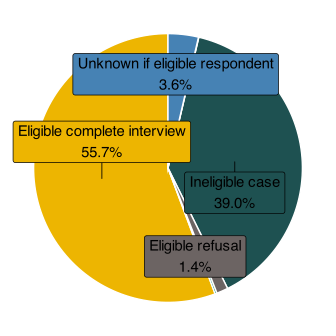
Table 4.2 summarizes typical survey durations and outcome frequencies for the core Gold Standard (GS)/NSUM/AS survey stream. Parallel summaries for RCM and LQAS are shown in Table 4.3 and Table 4.4. Although successful interviews are a minority of cases, they dominate total CAPI time. Ineligible cases are most common (48.4k; 59%), followed by completed interviews (22.5k; 27%). This reflects how listing and screening were integrated into the form, logging buildings and households separately. Accordingly, ineligible cases cover both non-qualifying households and listing work to identify buildings.
Yet completed interviews take much longer (45m 59s on average), so they dominate total time across all 22.5k cases. The right tail is long: one in five interviews exceeds 1h 03m 54s. Ineligible cases are shorter (8m 50s median; 14m 59s mean) but add up because they’re so frequent. Unknown eligibility cases comprise 10% (8m 08s average), while refusals and non-contacts are rare but still consume minutes per case. Overall, survey time is driven by frequent screen-outs and the long tail of lengthy interviews.
Code | Disposition Categorya | # Cases | Total | Median | Average | 80% Percentile |
|---|---|---|---|---|---|---|
I | Eligible complete interview | 22,501 | 718.4 | 0:41:18 | 0:45:59 | 1:03:54 |
NC | Eligible non-contact | 448 | 3.1 | 0:06:26 | 0:10:05 | 0:12:04 |
NE | Ineligible case | 48,351 | 503.1 | 0:08:50 | 0:14:59 | 0:25:03 |
R | Eligible refusal | 2,147 | 17.7 | 0:08:00 | 0:11:53 | 0:16:17 |
UH | Unknown if eligible household | 91 | 0.5 | 0:04:50 | 0:08:22 | 0:11:57 |
UO | Unknown if eligible respondent | 8,320 | 47.0 | 0:05:06 | 0:08:08 | 0:10:31 |
aCore survey refers to the integrated Gold Standard, NSUM, and initial Adaptive Sampling fieldwork stream. These components were implemented jointly in the field, so separating their time and cost cleanly is often analytically difficult. | ||||||
Code | Disposition Category | # Cases | Total | Median | Average | 80% Percentile |
|---|---|---|---|---|---|---|
Completed | Completed interview | 145 | 4.4 | 0:35:05 | 0:43:16 | 0:59:03 |
Missing | Not recorded | 90 | 0.3 | 0:01:54 | 0:04:42 | 0:03:26 |
Refused | Refused | 42 | 0.1 | 0:01:42 | 0:01:57 | 0:02:10 |
Non-contact | Non-contact | 25 | 0.0 | 0:01:12 | 0:01:56 | 0:02:27 |
NE | Ineligible case | 8 | 0.0 | 0:01:16 | 0:02:16 | 0:01:59 |
Code | Disposition Category | # Cases | Total | Median | Average | 80% Percentile |
|---|---|---|---|---|---|---|
Missing | Not recorded | 520 | 21.4 | 0:52:04 | 0:59:24 | 1:14:42 |
I | Eligible complete interview | 47 | 1.9 | 0:53:28 | 0:59:30 | 1:14:54 |
NE | Ineligible case | 21 | 1.1 | 0:55:06 | 1:12:40 | 1:20:56 |
R | Eligible refusal | 2 | 0.0 | 0:35:43 | 0:35:43 | 0:36:42 |
UO | Unknown if eligible respondent | 4 | 0.1 | 0:30:06 | 0:29:08 | 0:34:16 |
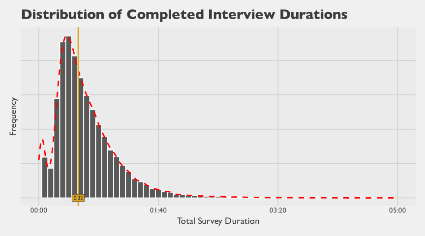
Figure 4.3 shows the distribution of interview duration for completed cases using frequency histograms with an empirical density overlay.1 Most interviews cluster at shorter times, while a smaller share run much longer, producing a right-skewed tail. This pattern is expected. There is a practical lower bound on interview duration, but field conditions–interruptions, case complexity, translation needs, and connectivity issues–can extend interviews unpredictably. A small number of long interviews absorbs a disproportionate share of time and drives variability in workload.
4.3.1.1.0.1 By Method
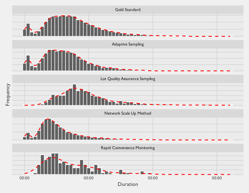
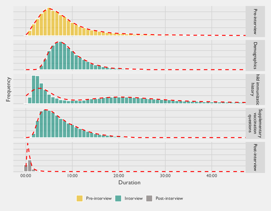
Figure 4.4 further decomposes this total time into key sections and shows that both central tendency and variability differ sharply across modules. Median durations are modest for post-interview steps (about 0m 37s), NSUM (2m 17s), and supplementary vaccination questions (6m 32s), while pre-interview tasks (7m 10s) and demographics (8m 23s) are more substantial. The child immunization history section stands out as the dominant time component (median about 16m 31s) and also exhibits the heaviest right tail, indicating that a minority of cases require much more time in this module. Taken together, the figures suggest that overall interview length is primarily driven by a mix of predictable fixed overhead (pre-interview and demographics) and highly variable case complexity concentrated in immunization history. For readability in this faceted distribution plot, the top 1% of durations within each section are trimmed.
Typical durations by survey section are summarized in Table 4.5 using the average, median, and 80th percentile2 for each section of the survey instrument.3
Average | Median | 80% Percentile | |
|---|---|---|---|
Pre-interview | 10M 24S | 7M 10S | 13M 6S |
Setup | 1M 38S | 44S | 1M 26S |
Geofenced GPS capture | 5M 9S | 2M 8S | 6M 34S |
Listing and building metadata | 1M 28S | 57S | 2M 15S |
Informed consent | 1M 59S | 1M 27S | 2M 51S |
Eligibility screening | 19S | 10S | 26S |
Demographics | 9M 20S | 8M 23S | 11M 55S |
Respondent demographics | 3M 25S | 2M 58S | 4M 30S |
HH characteristics | 5M 55S | 5M 8S | 7M 34S |
Child immunization history | 19M 46S | 16M 31S | 30M 46S |
Child immunization history | 19M 46S | 16M 31S | 30M 46S |
Supplementary vaccination questions | 7M 40S | 6M 32S | 10M 46S |
Cost of vaccination | 1M 50S | 1M 32S | 2M 36S |
Other | 49S | 34S | 1M 12S |
Access and barriers | 1M 23S | 1M 11S | 1M 55S |
KAP | 1M 54S | 1M 32S | 2M 46S |
Pathways Typing tool | 1M 14S | 1M 5S | 1M 42S |
NSUM | 2M 43S | 2M 17S | 4M 2S |
Post-interview | 1M 4S | 37S | 1M 13S |
Closeout | 1M 4S | 37S | 1M 13S |
Total | 39M 18S | 32M 58S | 55M 42S |
* Tabulated statistics comprise all successful interviews from the gold-standard and NSUM surveys, including the adaptive sampling study, but excluding the LQAS and RCM studies. | |||
Table 4.5 summarizes the mean, median, and 80th percentile for each section. Two points stand out. First, pre-interview time is substantial: median 7m 10s and mean 10m 24s, indicating a right tail. GPS capture dominates (2m 08s median, 5m 09s mean), with smaller shares for setup, metadata, and consent. Eligibility screening is negligible (seconds), so pre-interview time mostly reflects operational and documentation work, not screening.
Second, demographics takes a large share (8m 23s median, 9m 20s mean), driven mainly by household and respondent data, plus the typing tool. But immunization history dominates overall duration: 16m 31s median, 30m 46s at the 80th percentile. It accounts for the largest share of both typical length and the long tail. This makes sense: enumerators collect detailed histories for each child using home records when available, which increases effort and variability.
The child immunization history section shows the widest variation in duration, driven in part by the availability of Home-based records (HBRs). When enumerators could see the card, this module took a median of 24.2 minutes (n = 12,852 interviews); when the card was absent, the median was 3 minutes (n = 7,924). The difference reflects the fact that interviews with an available HBR require recording a more complete immunization history, including doses that may be omitted under caregiver recall, while also adding card-specific steps such as reviewing and photographing the card. This disparity also creates the potential for enumerators to discourage respondents from presenting the card, or even to misreport HBR availability, in order to substantially reduce interview time.
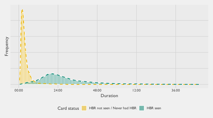
HBR Card Status | # Cases | Average | Median | 80th Percentile |
|---|---|---|---|---|
HBR not seen / Never had HBR | 7,924 | 4.5 | 3.0 | 5.1 |
HBR seen | 12,852 | 29.4 | 24.2 | 38.8 |
In sum, differences in total and survey length will therefore vary greatly on aspects like the number of children to be assessed, as well as other factors such as whether the sampled adult NSUM participant participated in the NSUM module.4 Figure 4.7 plots these average survey durations for different subsets of respondents.
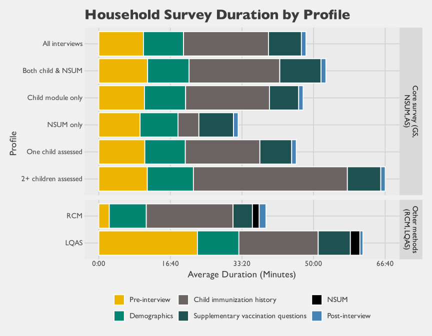
The LQAS bar shows a notably large pre-interview share compared to other methods. This reflects a design difference in the LQAS CAPI form: enumerators walked door-to-door within a lot until they completed a single interview with an age-eligible household, logging all screening activity within the same form instance. In contrast, enumerators using the other CAPI forms opened and closed a new form instance for each address attempted — whether or not it resulted in a completed interview — so that pre-interview screening time was distributed across many short instances rather than accumulated in one.
This survey time is both a draw on the time of the paid enumerator conducting the interview and on the respondent, who is not paid by the project for participating. From an economic perspective, respondent time carries an opportunity cost because those hours could otherwise be allocated to paid work, domestic production, care work, or other activities. Using the same time-audit traces, we can describe where those respondent-hours concentrate across household and interview profiles. The tabbed figures below show this concentration by wealth and employment, by Pathways type and employment, and by interview profile and employment. We then monetize those hours in the cost section.
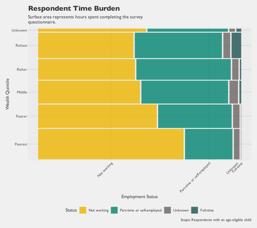
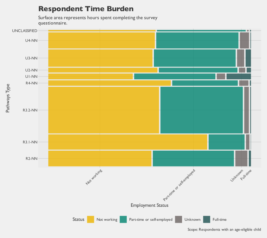
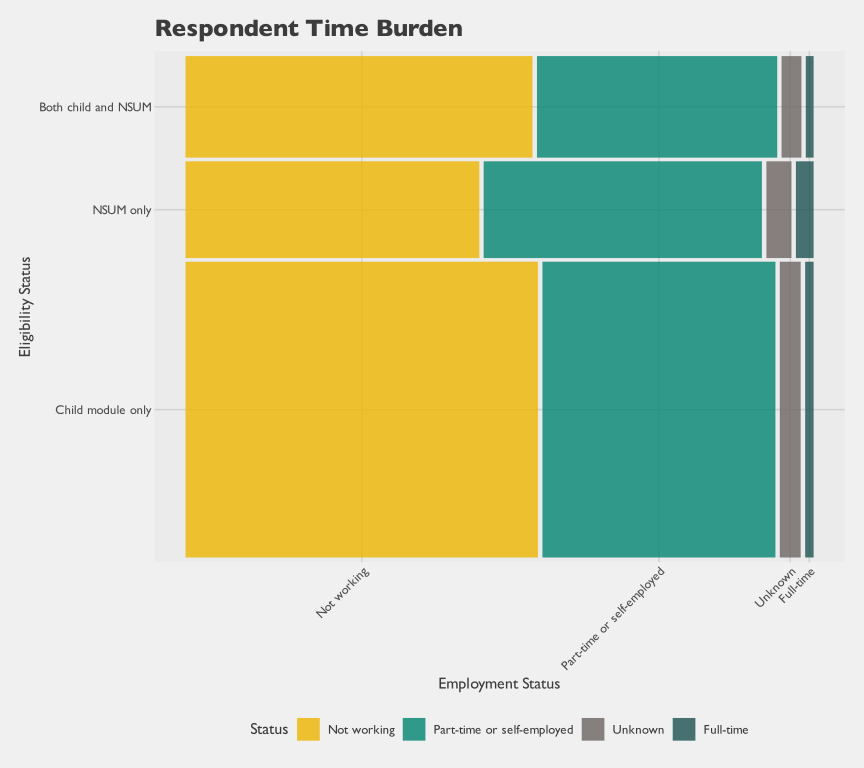
Figure 4.8 shows that respondent time is concentrated among people who report not working. Part-time or self-employed respondents account for most of the remaining hours. Full-time respondents contribute a much smaller share of total interview hours across wealth quintiles. This pattern is consistent with the Gold Standard sampling frame, which targets caregivers of infants and therefore tends to capture respondents with lower full-time labor-force attachment. Figure 4.10 shows that the NSUM-only interview profile has a somewhat higher share of fully employed respondents than profiles that include the child module, although this is still a small sliver of total respondent hours.
Method | Method Name | Interview Instances | Total Respondent Hours | Share of Total Respondent Hours |
|---|---|---|---|---|
GS | Gold Standard | 19,855 | 9,282 | 57.7% |
NSUM | Network Scale Up Method | 15,094 | 4,403 | 24.3% |
AS | Adaptive Sampling | 7,769 | 2,067 | 14.8% |
LQAS | Lot Quality Assurance Sampling | 594 | 508 | 2.7% |
RCM | Rapid Convenience Monitoring | 145 | 90 | 0.5% |
Beyond typical times, the CAPI data reveal how duration varies by enumerator, location, and stage of fieldwork. Because each action is timestamped and linked to a specific enumerator and location, duration changes can be tracked as enumerators gain experience. This shifts from static description to dynamics: where time goes, what slows or speeds interviews, and how teams improve with experience.
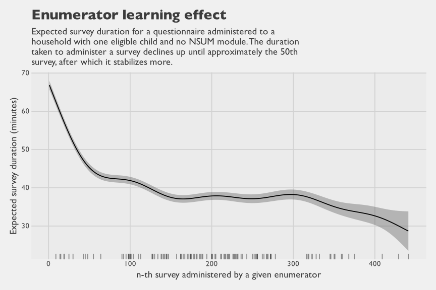
This analysis reveals economies of scale in survey administration time. Using local regression curves,5 survey duration decreases as enumerators gain experience. Figure 4.11 shows this: a typical enumerator spends 67 minutes on the first interview, 45 minutes by the 50th, and stabilizes around 38 minutes.6 Testing of other variables–training scores, prior experience–revealed that they added no predictive power.
While specific to this instrument and context, the learning curve is useful for planning: it quantifies predictable improvements that can be budgeted. Planners should treat duration as variable, not fixed. Build in ramp-up time: longer early interviews, structured training, and monitoring for stabilization, not day-one targets. The curve informs staffing and scheduling: how quickly to scale, how many interviews before steady-state productivity, and whether to address early inefficiency through coaching and logistics, not pressure.
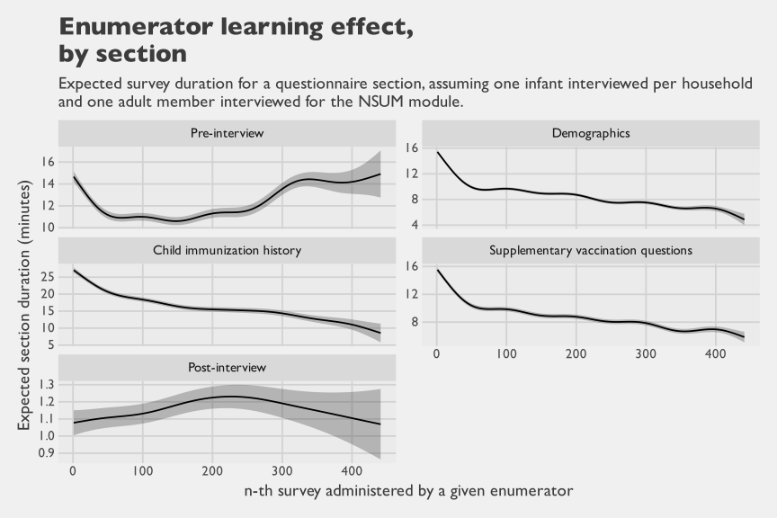
The learning curve summarises how the same enumerator’s expected duration evolves as they accumulate experience. The same multilevel model also estimates a random intercept for each of the 114 enumerators in the analysis, capturing how much an individual’s typical duration sits above or below the population mean once experience and case mix are accounted for.7 Figure 4.14 orders enumerators from fastest to slowest by their estimated deviation, with vertical bars marking ±1 conditional standard deviation around each estimate. The estimated between-enumerator standard deviation is roughly 8.7 minutes; the gap between the 10th and 90th percentile enumerators is approximately 18.3 minutes (from -9.1 to 9.2 minutes relative to the population mean) on a comparable interview, and the full range spans -15.6 to 34.8 minutes. Persistent between-enumerator differences of this magnitude sit alongside the within-enumerator learning effect: an experienced enumerator at the slow end of the distribution can take longer than a novice at the fast end on an otherwise identical interview.
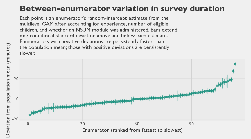
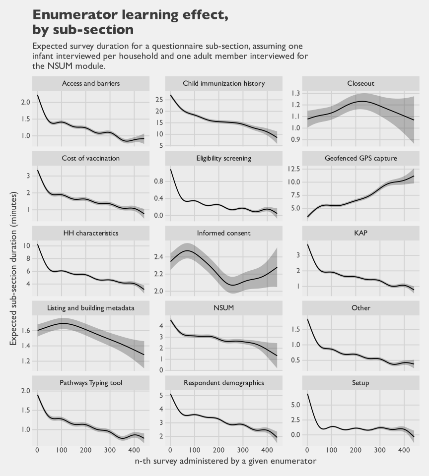
Figure 4.13 shows some noteworthy patterns by survey sub-section. While the time to administer subsections decreases for almost all subsections as enumerators progress along their fieldwork, the one clear exception is the time to capture GPS coordinates. This step involves both the task of finding the intended location as well as the task of recording GPS coordinates at a minimum level of accuracy (which can take time if cell reception is poor). While this step starts at approximately four minutes in duration when enumerators start conducing surveys, it gradually increases to approximately 10 minutes by the 300th interview. The most compelling explanation is that in a true probabilistic survey where units are pre-selected, it is common for more difficult cases to be skipped or abandoned by field teams who instead continue with neighboring areas that are easier to find. As the fieldwork progresses, mop-up visits are scheduled with more experienced and trusted enumerators who have proven their skill and competence by completing many other surveys. These skilled enumerators then complete previously missed/skipped cases, but may still find that this takes time as these cases may be more difficult to reach and may be in more remote areas where GPS systems are weaker. As the more difficult cases are re-attempted after initial failed attempts, this duration increase aligns with the enumerator’s experience.
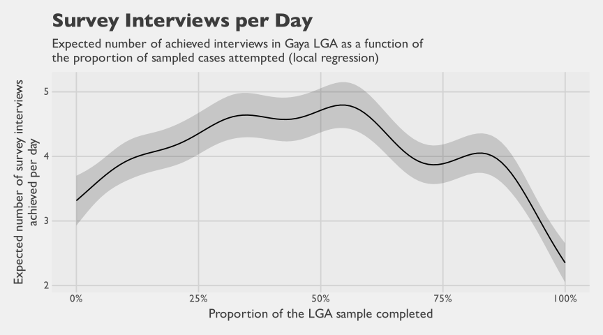
Enumerator learning effects do affect interview duration, but productivity does not increase monotonically over time. Field teams typically complete easier, more accessible cases first; more remote or otherwise difficult cases are deferred and often require repeat visits. Daily yields also fluctuate because eligibility and respondent availability are partly random, so teams may not complete all assigned cases within a day. This creates the need for “mop-up” work, where teams return to previously visited communities to finish a small number of outstanding interviews, increasing travel time and economic cost.
Figure 4.15 illustrates this pattern modeled for Gaya Local Government Area (LGA). A regression smoother8 shows successful interviews per day rising from roughly 3.5 early in fieldwork to about 4.5 midstream as teams gain familiarity, then falling to around 2.5 as remaining cases become more financially costly to complete near the end of data collection. These dynamics illustrate that implementers can sit at very different points on a spectrum of rigor and that this would have implications on time and financial cost. Teams running disciplined probability surveys incur a high financial tail cost from re-attempts and revisits needed to faithfully complete a predetermined sample, while convenience- or quota-based approaches often avoid that tail by substituting easier cases and/or moving on to the neighboring household, potentially introducing selection bias. The result is a structural difference in time and financial cost, and one that is directly linked to the validity of the realized sample.
The informed consent subsection in Figure 4.13 shows a noisier pattern than most other sections. Its error bands are wider largely because this is a very short activity, so small absolute differences translate into larger relative uncertainty, as with other brief steps such as listing and closeout. The fitted trend also suggests a possible increase after roughly 200 interviews, but the uncertainty intervals are wide enough that this could easily be a spurious pattern. A plausible alternative explanation is selection: the most competent enumerators are often assigned harder late-stage cases, and those respondents may require more time and explanation before consenting.
4.3.1.2 Field Time
Field time tracks an enumerator’s workday outside the survey form. It follows a sequence of operational checkpoints: leaving home, meeting at an assembly point, traveling to the Enumeration Area (EA), leaving the EA at the end of the day, and returning home. This captures travel and coordination at a scale useful for planning and budgeting.
Enumerators logged checkpoints throughout the day using a CAPI form that captured timestamps, GPS, and vehicle mileage. Because logging was manual, these data are semi-self-reported and prone to missingness or timing errors compared to system-generated timestamps. However, the form was designed to prevent errors: checkpoint times defaulted to current time, GPS was captured automatically, and logic blocked impossible sequences (leaving home after arrival, for example). These safeguards ensured that the data remained clean for day-level analysis.
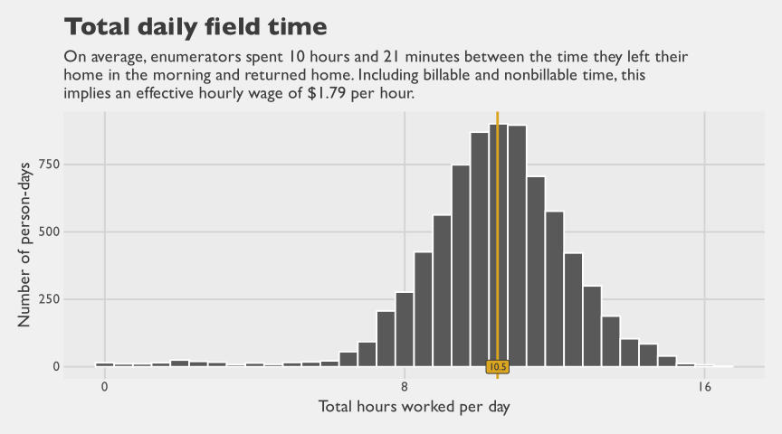
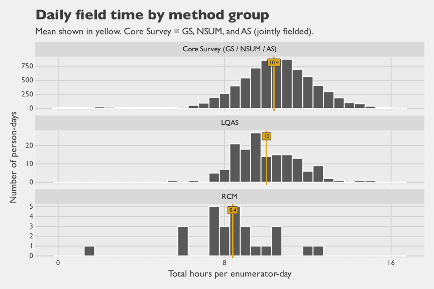
The daily work-time distribution in Figure 4.16 pools all enumerator-days across the study. Because GS, NSUM, and AS were fielded jointly as a single integrated operation (March 2024–July 2025) with shared logistics, their enumerators share the same daily time profile — referred to here as the Core Survey group. LQAS and RCM were fielded separately (May 2025–July 2025) under distinct operational arrangements; their enumerators’ daily time profiles may therefore differ from the Core Survey. For ARR, enumerators did not complete time-motion forms for the Primary Health Center (PHC) data collection method. A typical administrative method would also be largely desk-based rather than field-based. We therefore exclude ARR from the method-specific estimates.
The Core Survey and LQAS distributions look broadly similar. The RCM distribution is different: enumerators spent an average of 8.4 hours per day, which is much closer to the expected 8-hour workday. That pattern is consistent with the operational design. RCM field workers did not move in teams, so they did not face the same delays from waiting for colleagues to finish interviews. Because RCM used a convenience sample that moved from one nearby household to the next, enumerators also likely spent less time traveling between locations. Nevertheless, not all RCM field days ended at or shortly after 8 hours. Some extended well beyond that point, while others were considerably shorter. The shorter days likely reflect enumerators reaching the 20-child target for that RCM round. The reasons for the longer RCM days are less clear.
Method Group | Enumerator-Days | Mean (hrs)† | Median (hrs) | SD (hrs) |
|---|---|---|---|---|
Core Survey (GS / NSUM / AS) | 7,461 | 10.37 | 10.49 | 2.06 |
LQAS | 157 | 10.01 | 9.73 | 1.55 |
RCM | 27 | 8.39 | 8.36 | 2.08 |
†37 enumerator-days in the time-motion data matched to more than one survey method via enumerator ID and date. These mixed days are excluded from per-method distributions and the method summary table. | ||||
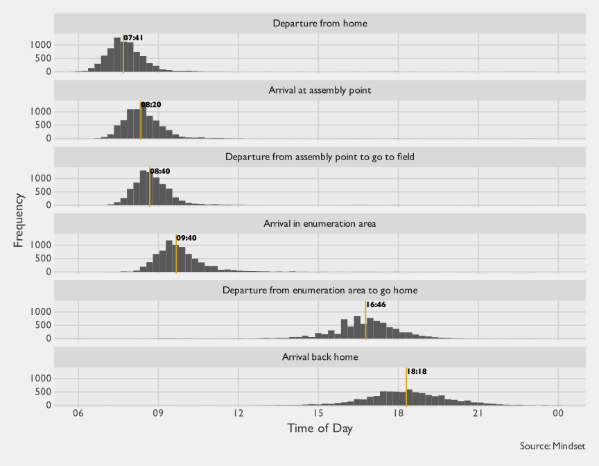
Figure 4.18 shows when the typical workday began and ended: enumerators left home at 07:41, met the team at 08:20, and departed for the field at 08:40. Table 4.9 then shows how that day was allocated across steps. Enumerators typically spent 7 hours in the EA, but the full workday stretched beyond that once travel and coordination time were included. Morning times were consistent, but end-of-day times varied widely.
Three factors likely explain this end-of-day variability. First, teams typically start the day at a fixed time, but they account for travel time when deciding when to leave the EA. Teams working in more distant EAs often wrap up fieldwork early to allow enough time to return home. Second, teams may extend the day slightly if only one or two scheduled surveys remain in the EA, to avoid making a return visit. Third, although teams can depart immediately in the morning, they often must wait at the end of the day for in-progress interviews to finish before returning home. A typical team consists of a driver and three enumerators; if two enumerators finish near the target end time but the third has just started a 45-minute interview, the others must wait. Together, these factors make return time less predictable.
Step | Median | Mean | 80% | Standard | 50% Highest Density Interval | Weibull fit | ||
|---|---|---|---|---|---|---|---|---|
Lower bound | Upper bound | Shape | Scale | |||||
Travel to assembly point | 35 min | 39 min | 56 min | 27 min | 14 min | 41 min | 1.85 | 43.04 |
Waiting time at assembly point | 14 min | 22 min | 36 min | 30 min | 0 min | 14 min | 1.05 | 22.98 |
Travel time to enumeration area | 54 min | 63 min | 90 min | 57 min | 13 min | 61 min | 1.44 | 68.60 |
Fieldwork in enumeration area | 7.0 hours | 6.9 hours | 8.0 hours | 94 min | 6.1 hours | 7.7 hours | 5.70 | 443.73 |
Travel time to go home/hotel | 87 min | 96 min | 2.2 hours | 67 min | 44 min | 103 min | 1.92 | 106.96 |
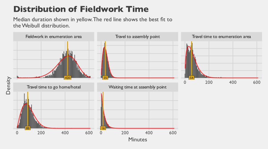
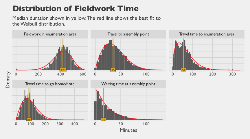
Table 4.9 is the main summary table for the enumerator workday. It shows that the day was dominated by work in the EA: the median time in the field was 7 hours, with a mean of 6.9 hours. The 50% Highest Density Interval (HDI) shows where the middle half of durations clustered, which for fieldwork was 6.1 hours to 7.7 hours. The 80th percentile helps show the upper-tail burden relevant for staffing and transport planning: fieldwork reached 8 hours, and travel home reached 2.2 hours.
The table also shows that total day length was not driven by interviewing alone. Travel to the EA typically took 54 min, while the return trip home was longer at 87 min and more variable. Waiting at the assembly point was smaller, with a median of 14 min, so it contributed less to day length than either travel segment or in-EA work.
Figure 4.20 shows the same data as histograms with Weibull curves overlaid. Weibull distribution is used because duration data are positive and right-skewed; it captures both the bulk and tail with two parameters.
4.3.1.3 Project Time
Total staff time across the entire project was compiled, including enumerators, permanent staff, and consultants across all phases: planning, data collection, quality control, analysis, and dissemination.
Multiple sources contributed to this compilation. For consultants, billed hours were converted to Level of Effort (LOE), with one LOE unit representing an 8-hour day; for field teams, days were recorded at their daily rate; for permanent staff, budgeted allocations were cross-checked against self-reported time by phase and method, and discrepancies were resolved with finance, aligning permanent-staff totals to reported time.
Allocation detail varies by person and role. For some–consultants with timekeeping software–breakdowns are precise. For others, recall and estimates were used. Total LOE by cadre is well-supported; method-level breakdowns are approximate.
Many activities were shared across methods, especially common research infrastructure. Developing the survey instrument supported all but one method; this work could not be attributed to any single approach. Training had the same pattern. Although some methods required shorter refreshers or protocol-specific components (for example, RCM walk procedures versus pre-selected household visits in the Gold Standard design), much of training time covered shared questionnaire administration, field protocols, and logistics used across methods. Therefore, an ‘All methods’ category was created for shared time.
Two approaches were used to allocate shared time and cost by method. For field teams, time was split proportionally to successful interviews. Field time for NSUM, GS, and AS was split by the proportion of interviews for each. For staff, ‘All methods’ time was split proportionally to their reported allocation for other categories. For instance, if someone reported 2 days as ‘All methods’, 4 for NSUM, and 6 for RCM, the 2 days would be split as follows: 40% to NSUM, 60% to RCM.
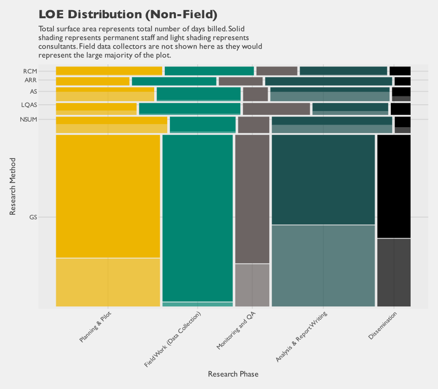
Figure 4.21 shows staff by method and employment. Mosaic plots visualize two categorical variables: the width of each slice shows the frequency of one variable, and the height of rectangles within it shows conditional proportions of the other. Area represents share of observations, so larger blocks mean more cases. Similarities across slices suggest independence; shifts suggest association.
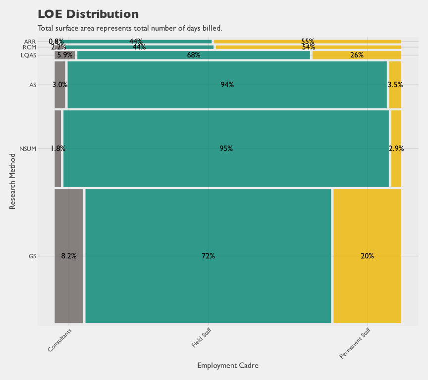
Field teams dominate: roughly three-quarters of overall effort, consistently across methods. Consultants and permanent staff take a larger share in Gold Standard and LQAS.
To see differences among non-field staff, Figure 4.22 excludes field teams and breaks effort by phase. Non-field time spreads more evenly across phases, with smaller shares for monitoring, Quality Assurance (QA), and dissemination. Phase shares are stable across methods, but consultants contribute less to collection and QA, more to analysis and dissemination.
4.3.2 Cost
Expenditures cover transactions from 2023-04-13 to 2025-12-25. Because nomenclature differs across studies and industries, we stipulate definitions up front and use them consistently throughout. The analyses are organized using two cost distinctions: financial versus economic and total versus marginal. These dimensions clarify both what resources are counted and how costs change as output scales.
The first dimension is about what is counted in furtherance of the research work. Financial cost is what can be traced back to Mindset’s accounting ledger (expenditures, amortization, and other allocated charges). Non-financial cost captures resources consumed that do not appear in Mindset’s ledger, including unpaid staff overtime, unbilled consultant time, and time contributed by stakeholders such as government officials. In principle, definitions of non-financial cost can be broader still, for example including the opportunity cost to respondents of participating in the survey. This chapter includes an estimate of respondent opportunity cost using observed questionnaire duration and respondent socioeconomic proxies. In this study, the sum of financial and non-financial costs is termed the economic cost, reflecting the full mix of paid and unpaid resources required to complete the research.
The second dimension is about what change is being measured. Total cost is the full resource burden of delivering a method at the observed scale, expressed as a summation of costs. Marginal cost is the additional cost of producing one more unit of research output holding fixed costs constant (for example, an additional child measured, household interviewed, or cluster). In practice, marginal cost is an average cost over a specified number of units of output. Marginal cost multiplied by quantity provides a simple variable-cost approximation, which, when added to fixed costs, recovers the corresponding total cost.
\[ \text{Total Cost} \approx \text{Fixed Cost} + \textrm{Unit Quantity} \times \text{Marginal Cost} \tag{4.1}\]
Table 4.10 summarizes the terminology and provides concrete examples for each quadrant.
(A) | (B) | (A + B) | |
|---|---|---|---|
Financial Cost | Non-financial Cost | Economic Cost | |
Total Cost | Total financial cost consists of the sum of (i) cash expenditures and (ii) amortized capital costs, both taken from Mindset's accounting records and, where needed, fractionally allocated to methods or implementation phases. Matches what the accounting ledger would show for the method at the study scale. Example components: Wages, salaries, fuel costs, amortization of electronic tablets | Total non-financial cost comprises resources consumed in furtherance of the research but not paid by Mindset. Examples: enumerator travel time from/to home; overtime beyond the presumptive 8-hour day; government stakeholder time in meetings; unbilled consultant support; respondent opportunity cost of participation. | Total economic cost comprises the total financial cost plus the total non-financial cost. It is interpreted as the full resource burden of delivering the method at the study scale. |
Marginal Cost | Marginal financial cost is the expected (i.e., average) per-unit expenditure needed to add one more unit of output (one more respondent, one more cluster, etc.). | Marginal non-financial cost comprises expected resources consumed but not paid by Mindset for every additional unit of output. Examples: enumerator overtime (beyond 8 hours). In this chapter, we also include respondents' opportunity cost of participation. | Marginal economic cost is the expected (i.e., average) per-unit resources needed to add one more unit of output, whether borne to Mindset or not. Interpreted as the incremental resource burden of scaling output. |
A third dimension concerns budgeted versus actual costs. We do not emphasize this distinction here because we do not compare budgets to actuals; all results in this section use actual costs.
Each dimension has its own utility. A budget-to-actuals comparison is most useful for assessing how well plans matched reality, and for quantifying cost uncertainty and the risk of under-budgeting. Within the actual-cost framework used here, total financial cost is most informative for how donors and implementers can price and contract for studies of this type, since it reflects realized expenditures; unit costs can still vary materially with scale and scope. For that reason, marginal cost complements total cost for forward planning and scale-up scenarios, because it approximates how total cost changes with output and helps separate fixed overhead from the additional resources required to add interviews, clusters, or field-days. Finally, total economic cost helps characterize the full resource burden, including unpaid and externally borne time costs.
4.3.2.1 Total Cost
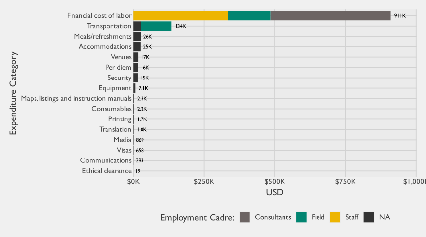
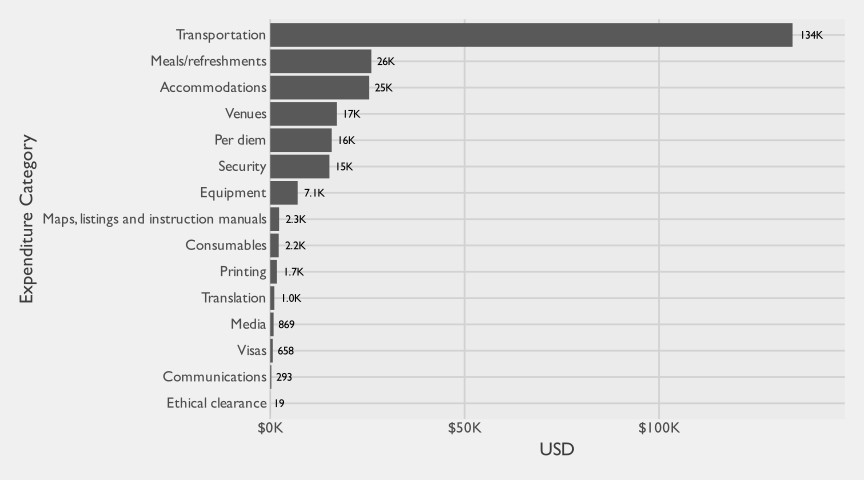
Figure 4.23 displays total financial costs by category.9 Labor dominates: $910,676, representing 78% of total and substantially exceeding all other categories.10 Figure 4.24 shows the same breakdown with labor removed, making the smaller non-labor categories easier to compare. Most of these non-labor costs are shared overhead, allocated proportionally to successful interviews by method (Table 4.1). Exceptions include EA map acquisition (specifically for LQAS).
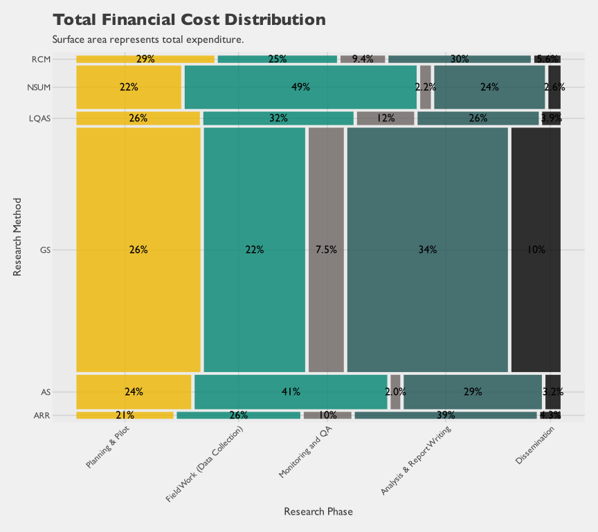
The next breakdown shifts from cost category totals to where those costs were incurred in field implementation. It decomposes financial spending jointly by method and research phase to show how each method draws on setup, training, and implementation activities.
method | Planning & Pilot | Monitoring and QA | Analysis & Report Writing | Field Work (Data Collection) | Dissemination | Total |
|---|---|---|---|---|---|---|
GS | $210,706 | $47,550 | $218,123 | $188,647 | $107,198 | $772,224 |
NSUM | $57,150 | $2,515 | $26,543 | $94,500 | $3,020 | $183,728 |
LQAS | $11,497 | $4,171 | $8,865 | $16,238 | $1,340 | $42,111 |
AS | $38,849 | $1,786 | $26,316 | $55,109 | $2,932 | $124,991 |
ARR | $3,730 | $1,757 | $6,738 | $4,582 | $749 | $17,557 |
RCM | $5,716 | $1,746 | $5,604 | $6,053 | $1,033 | $20,152 |
Total | $327,648 | $59,524 | $292,189 | $365,130 | $116,272 | $1,160,763 |
The table reports the rounded USD values. Because shared analytic and operational effort within the core survey (gold standard, NSUM, and AS) was apportioned across these methods in proportion to successful interview counts, the phase totals index allocated spend per method rather than per-unit analytic or operational difficulty. In particular, the lower analysis-phase spend shown for AS than for the gold standard does not imply that AS is analytically simpler: AS builds on the gold standard’s sample frame, weights, and design-based variance estimation, and a standalone implementation would have to carry that infrastructure on its own. The mosaic that follows emphasizes composition by plotting each method’s phase shares as proportional area.
The integrated summary below consolidates economic costs, counts, and per-unit averages in one table.
label | GS | NSUM | AS | LQAS | RCM | ARR |
|---|---|---|---|---|---|---|
Economic Costs | ||||||
A. Permanent Staff & Consultants | $573,194 | $63,764 | $60,077 | $30,680 | $17,524 | $16,099 |
B. Field staff (economic cost) | $146,161 | $110,532 | $60,249 | $11,487 | $3,004 | $1,684 |
C. Stakeholder (gov't) and respondents | $4,621 | $1,359 | $829 | $150 | $27 | $0 |
D. Non-labor cost (expenditures + amortization) | $134,162 | $70,908 | $35,500 | $7,713 | $1,647 | $157 |
Total economic cost (A + B + C + D) | $858,137 | $246,563 | $156,656 | $50,030 | $22,202 | $17,941 |
Counts | ||||||
Number of Respondents (Households) | 21,525 | 16,278 | 8,649 | 594 | 145 | 74 |
Number of Clusters | 1,814 | 1,747 | 330 | 594 | 8 | 74 |
Averages | ||||||
Average Cost/Respondent (HH) | $40 | $15 | $18 | $84 | $153 | $242 |
Average Cost/Cluster | $473 | $141 | $475 | $84 | $2,775 | $242 |
Table 4.12 reports economic costs, defined here as the sum of financial and non-financial costs, including costs not borne by Mindset. The grouped rows highlight three patterns. First, labor dominates total economic cost, with permanent staff and consultants forming the largest component for most methods and field labor adding a substantial second layer. Second, the stakeholder and respondent component is smaller in dollar terms but still non-negligible, making explicit that implementation draws on unpaid time outside Mindset’s financial ledger. Third, average cost per respondent and per cluster depends strongly on scale. Methods with small operational footprints can show higher per-unit costs because fixed and semi-fixed effort is spread over fewer completed units. RCM illustrates this most clearly: at $2,775 per cluster and $153 per household, its averages are well above those of the other methods, but the underlying drivers are denominator effects rather than expensive fieldwork. The design covered only 8 facility catchment areas (two per stratum), and the pseudo-random walks produced roughly 18 completed households per facility, so fixed overhead, training, supervision, travel, and the geospatial work needed to define each walk corridor are amortized over very small denominators. At the margin, by contrast, RCM costs $16 per additional household and $14 per child assessed—broadly in line with the field rates seen for the larger methods (see Table 4.21). For interpretation, total and average metrics should therefore be read together rather than in isolation.
4.3.2.2 Cost of Labor
Labor is the largest cost and merits detailed attention. The distribution of time across activities and roles is examined, along with how that drives differences in cost and efficiency.
4.3.2.2.1 Financial cost of labor
Figure 4.26 shows financial labor cost by method and cadre.
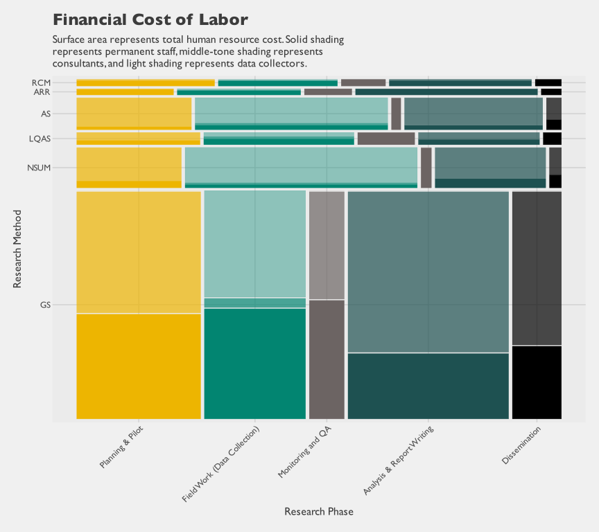
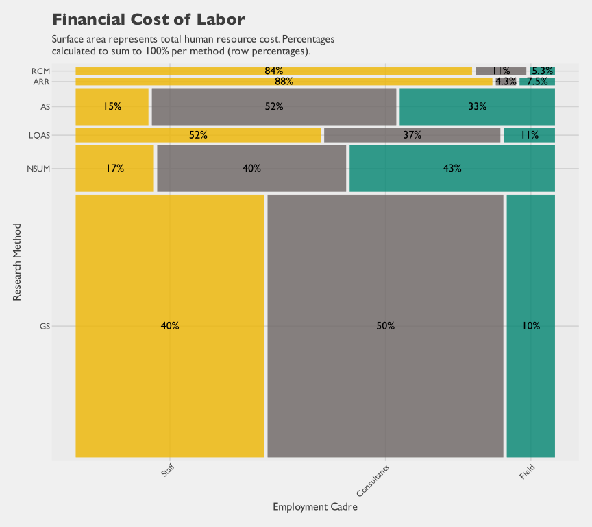
Figure 4.27 shows the same data differently, emphasizing method-by-cadre patterns: NSUM and adaptive sampling used more consultants; RCM and ARR relied more on permanent staff.
4.3.2.2.2 Non-financial cost of labor
Direct and indirect labor costs can be examined. Direct costs capture billable time; indirect costs capture hidden time (unbilled hours, uncompensated participation). This includes unbilled consultant hours, stakeholder time (e.g., government employees), and fieldwork time beyond the 8-hour assumption.
For enumerators, the nominal wage was calculated as $18.50 per day divided by 8 hours, yielding $2.31 per hour. However, actual fieldwork time (including travel to and from home) averaged 10.36 hours per day. As Table 4.9 shows, only 7 hours of a typical day was spent in the EA; the remainder reflected travel to the assembly point, waiting, travel to the EA, and the longer trip home. Dividing the daily wage of $18.50 by those actual hours yields the lower effective hourly wage of $1.79.
The effective hourly wage varies by method because GS/NSUM/AS, LQAS, and RCM were fielded under different operational arrangements with potentially different daily field durations. Table 4.14 shows the method-specific effective wages derived from matched time-motion data.
Type | Components | Formula | Amount (USD) |
|---|---|---|---|
Nominal hourly wage | billable | $18.5 per day / 8 hours | $2.31 |
Effective hourly wage | billable + non-billable | $18.5 per day / 10.36 hours | $1.79 |
Method | Time-Motion Group | Enumerator-Days | Mean Daily Hours | Nominal Wage (USD/hr) | Effective Wage (USD/hr) |
|---|---|---|---|---|---|
Gold Standard | Core | 7,461 | 10.37 | $2.31 | $1.78 |
NSUM | Core | 7,461 | 10.37 | $2.31 | $1.78 |
Adaptive Sampling | Core | 7,461 | 10.37 | $2.31 | $1.78 |
LQAS | LQAS | 157 | 10.01 | $2.31 | $1.85 |
RCM | RCM | 27 | 8.39 | $2.31 | $2.21 |
Table 4.15 compares the two: the direct financial cost of $257,178 increases substantially to $332,448 when hidden enumerator time is included, using method-specific field hour estimates.
Method | Billable hours | Non-billable hours | Time-motion-adjusted hours | Financial cost | Non-financial cost | Total economic cost | Mean field hours |
|---|---|---|---|---|---|---|---|
GS | 28,051 | 8,316 | 36,368 | $112,841 | $33,454 | $146,295 | 10 |
NSUM | 21,213 | 6,289 | 27,502 | $85,335 | $25,299 | $110,634 | 10 |
AS | 12,719 | 3,771 | 16,490 | $46,514 | $13,790 | $60,304 | 10 |
LQAS | 1,608 | 405 | 2,013 | $8,868 | $2,231 | $11,100 | 10 |
RCM | 424 | 21 | 445 | $2,320 | $113 | $2,432 | 8 |
ARR | 416 | 123 | 539 | $1,300 | $384 | $1,684 | 10 |
Total | 64,432 | 18,924 | 83,356 | $257,178 | $75,270 | $332,448 |
Stakeholder time also contributes meaningfully to total labor input, especially from government agencies participating in training, engagement, supervision, and technical sessions. To make those contributions visible, we summarize stakeholder-reported hours and their implied USD value using the stakeholder costing target. In the terminology used in this report, stakeholder labor is a non-financial cost when it is not paid by Mindset but is still required to execute the work. When that time is valued in USD, it contributes to economic cost rather than direct financial cost.
Mindset attempted to quantify this non-financial stakeholder contribution using project records. The Mindset project manager estimated stakeholder-by-stakeholder participation time from meeting minutes, attendance records, training records, and related engagement documentation. For government stakeholders, role-linked pay scales are publicly accessible, so time could be valued using salary levels aligned to the reported role grade. Those values are treated as economic opportunity cost rather than financial expenditure, because Mindset did not directly pay those government salaries. In total, stakeholders contributed an estimated 971 hours of non-financial labor input, valued at approximately $1,401 in economic-cost terms across 45 individuals from 8 organizations. Most of this value came from government participants, who accounted for 99.4% of the estimated stakeholder USD contribution. For reporting stability, agencies with fewer than five observations are grouped into an “other” category, yielding 3 agency groups in the table below. The largest contributing named agencies were the State Primary Health Care Management Board (SPHCMB) and Kano Bureau of Statistics (KNBS). These results indicate that stakeholder participation was not limited to nominal attendance. Reported time concentrated in operationally relevant activities such as training and monitoring, engagement meetings, technical sessions, and dissemination support.
Contributor Type | Agency | Individuals | Total Hours | Estimated Economic Value (USD) | Share of Stakeholder Value |
|---|---|---|---|---|---|
Government | SPHCMB | 32 | 621 | $1,080 | 77.0% |
Government | KNBS | 7 | 280 | $200 | 14.3% |
Government | Other | 5 | 65 | $113 | 8.1% |
Non-government | Other | 1 | 5 | $8 | 0.6% |
The agency table identifies who contributed the largest share of stakeholder time. The activity table then shows what that time was used for. Most engagement time was concentrated in meetings and coordination activities, with training also representing a meaningful secondary share.
Primary Activity | Individuals | Total Hours | Estimated Economic Value (USD) | Share of Stakeholder Value |
|---|---|---|---|---|
Engagement Meeting | 38 | 691 | $1,201 | 85.7% |
Training/Monitoring | 7 | 280 | $200 | 14.3% |
Respondent time is also a non-financial input to the study. The 37,529 completed interviews in this costing set account for 17,909 respondent hours in total. From an economic perspective, these hours represent respondent opportunity cost. That opportunity cost is not identical across households and is not limited to observed cash earnings. Many respondents are women with limited formal labor-force participation, but their time still has substantial economic value through childcare, household production, and other unpaid work. Estimating household-specific non-market time value is a separate research exercise, so this chapter uses a simpler, transparent, tractable valuation rule for comparative costing. The base hourly benchmark uses the NGN 70,000 federal minimum monthly wage (National Salaries, Incomes and Wages Commission (NSIWC) (2024)), converted to hourly terms and then adjusted by wealth quintile.11 Wealth multipliers are calibrated to national deflated consumption quintile means from the Nigeria Living Standards Survey (NLSS) 2019–2020 (National Bureau of Statistics (NBS) (2020)), normalized to the middle quintile. Because the household wealth index is estimated from the completed child-module household frame, many NSUM-only interviews do not have an estimable wealth quintile and are classified as unknown in these respondent-cost summaries.
Wealth Quintile | Multiplier |
|---|---|
Poorest | 0.438x |
Poorer | 0.715x |
Middle | 1.000x |
Richer | 1.400x |
Richest | 2.615x |
Unknown | 1.000x |
The assumptions table is intentionally narrow and only reports the wealth multipliers used in the base valuation. The next table applies those multipliers to observed respondent minutes and reports the resulting implied economic values overall and by method.
Method | Method Name | Completed Interviews | Respondent Hours | Estimated Economic Value (USD) | Implied USD per Hour | Share of Respondent Valueb |
|---|---|---|---|---|---|---|
ALL | All methods (total) | 37,529 | 17,909 | $6,053 | $0.34 | 100.0% |
GS | Gold Standard | 19,855 | 9,282 | $3,228 | $0.35 | 57.7% |
NSUM | Network Scale Up Method | 15,094 | 4,403 | $1,359 | $0.31 | 24.3% |
AS | Adaptive Sampling | 7,769 | 2,067 | $829 | $0.40 | 14.8% |
LQAS | Lot Quality Assurance Sampling | 594 | 508 | $150 | $0.29 | 2.7% |
RCM | Rapid Convenience Monitoring | 145 | 90 | $27 | $0.30 | 0.5% |
bMethod shares are normalized across method rows and sum to 100%; overlapping interviews/modules are apportioned across methods. | ||||||
Table 4.19 apportions respondent time across interview modules and reports both the all-method total and method-specific values in one table. When a completed case contains both child and NSUM interviews, time is split equally across those two modules for method-level accounting.
Wealth Quintile | Completed Interviews | Respondent Hours | Estimated Economic Value (USD) | Share of Base-Scenario Value |
|---|---|---|---|---|
Richest | 3,880 | 2,586 | $1,996 | 33.0% |
Richer | 3,280 | 2,101 | $868 | 14.3% |
Middle | 3,690 | 2,325 | $686 | 11.3% |
Poorer | 4,011 | 2,385 | $503 | 8.3% |
Poorest | 5,420 | 3,097 | $400 | 6.6% |
Unknown | 17,248 | 5,416 | $1,599 | 26.4% |
As discussed in Section 4.4.3, these USD valuations should be interpreted as exchange-rate contingent. They are useful for cross-method comparability in a single reporting frame, but macroeconomic shifts in the naira can materially change the USD expression of the same local-currency effort.
4.3.2.2.3 Total economic cost of labor
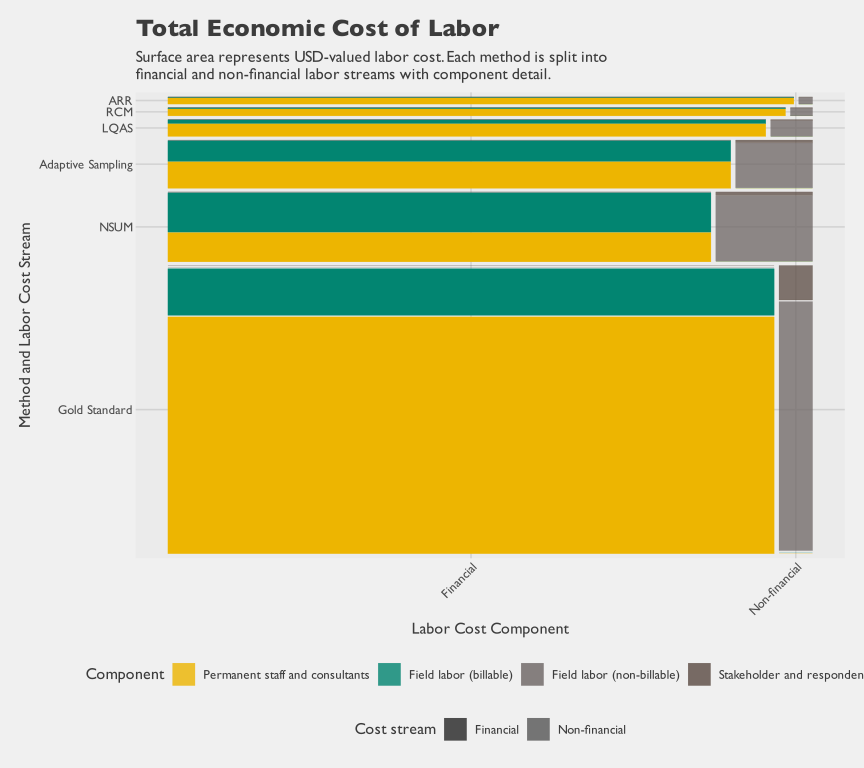
Financial and non-financial labor costs can be read together as total economic labor cost. For each method, we combine:
- permanent staff and consultant labor (financial),
- direct billable field labor (financial),
- hidden field labor from non-billable time (non-financial), and
- stakeholder and respondent opportunity cost (non-financial).
Figure 4.28 shows how the composition shifts across methods. Across all methods combined, financial labor remains the larger share, while non-financial labor still contributes a visible portion of total labor cost.
4.3.2.3 Marginal Cost
Previous sections reported total and average costs. However, averages incorporate fixed costs (questionnaire design, overhead) that do not scale with sample size. Marginal costs isolate what actually scales: the variable field effort to interview additional cases and visit additional clusters. These support future planning and scenarios.
Table 4.21 reports marginal costs per additional child, household, and cluster. It also reports per-LGA averages of the same direct field costs, to support coarser, funder-oriented budget comparisons. These isolate variable field costs–what actually changes with sample size–excluding fixed components like planning, training, programming, and analysis.
Marginal rates should be interpreted as averages, not constants. Fieldwork speed varies: teams accelerate after training, then slow again near the end (mop-up work). Despite this variation, marginal costs are useful for planning: they enable estimation of variable costs for different sample sizes.
Unit-level costs do not differ substantially across methods. Large differences in total cost arise from sample size and operational scope, not marginal rates. This distinction is important for planning: resource constraints and precision goals may imply very different sample sizes than those used in this study. For an interactive planning tool that integrates empirical findings from this chapter with sample size assumptions to estimate expected cost, see the sample-size calculator in Appendix B. For adaptive sampling, the row labeled “Adaptive Sampling (Supplement)” in Table 4.21 represents only the adaptive supplement (the additional hotspot-directed visits after the initial sample). The initial sample draw is grouped under the core survey because those households were visited through the same shared Gold Standard + NSUM fieldwork that also generated the hotspot inputs for adaptive targeting.
Method | Level of Effort for Field Staff | Marginal Financial Costa | Children Assessed | Households Interviewed | Clusters Visited | Children Assessed per Cluster | Marginal Financial Cost per... | ||||||||
|---|---|---|---|---|---|---|---|---|---|---|---|---|---|---|---|
12-23 mo | 0-23 mo | Child | Child | HH | Cluster | Lot | LGA | Facility | RCM | ||||||
days | USD | # | # | # | # | # | USD | USD | USD | USD | USD | USD | USD | USD | |
Core (Conventional + NSUM) | 7,408 | $238,400 | 11,263 | 23,617 | 21,525 | 2,097 | 11.3 | $10.09 | $21.17b | $11.08 | $113.69 | $15,893.33 | |||
Adaptive Sampling (Supplement) | 340 | $6,290 | 531 | 1,063 | 976 | 45 | 23.6 | $5.92 | $11.85b | $6.44 | $139.78 | $524.17 | |||
LQAS | 201 | $8,868 | 594 | 594 | 594 | 1.0 | $14.93 | $14.93 | $14.93 | $277.14 | $2,956.17 | ||||
RCM | 53 | $2,320 | 167 | 145 | $13.89 | $16.00 | $331.36 | $289.94 | |||||||
ARR | 52 | $1,300 | $76.47 | $17.57 | |||||||||||
aMarginal financial costs include wage payments made to enumerators and supervisors for field work related to listing, interviewing, and quality assurance. It includes costs for travel and accommodation necessary for field work, but excludes training costs for field staff, and excludes overhead. | |||||||||||||||
bMarginal costs for children 12-23 for the core and adaptive sample are over-estimates, as they do not net out costs incurred by enumerators assessing children aged 0-11 months. | |||||||||||||||
cLGA denominators reflect each method's design scope. LQAS's n=3 covers only the sentinel LGAs by design. ARR's n=17 includes the 15 study LGAs plus 2 (Kano Municipal and Makoda) that were withdrawn from the study after data collection had already begun. | |||||||||||||||
4.3.3 Precision
The decision objective is to compare methods on accuracy relative to resource use. Accuracy, however, has two components: bias and precision. Bias reflects systematic error and does not necessarily improve with larger sample sizes. Precision reflects random sampling error and does improve predictably as sample size increases.
For this comparison, we treat the Gold Standard as the best available benchmark against which the other methods are evaluated. Among the methods studied, it has both the most extensive protocols for limiting bias and a sample large enough to make the resulting estimate highly precise; together these properties make it the closest available approximation to true coverage. No household survey is entirely free of instrumentation or recall error, but the alternatives here depart from plausibility by a different order of magnitude: ARR can imply coverage above 100% in some clusters, and NSUM estimates diverge substantially from the Gold Standard. The precision-cost analysis that follows therefore focuses on the Gold Standard, whose larger sample also supports the more detailed analyses; under explicit assumptions, it asks how much uncertainty can be reduced for a given budget. The NSUM precision curves are shown for theoretical context, but they are not the basis of the planning conclusions that follow. A useful starting point is the theoretical relationship between precision and sample size under negligible bias. Figure 4.29 isolates sampling error and shows how margins of error decline as sample size increases under different design-effect assumptions. This establishes a baseline from statistical theory before the next subsection adds cost.
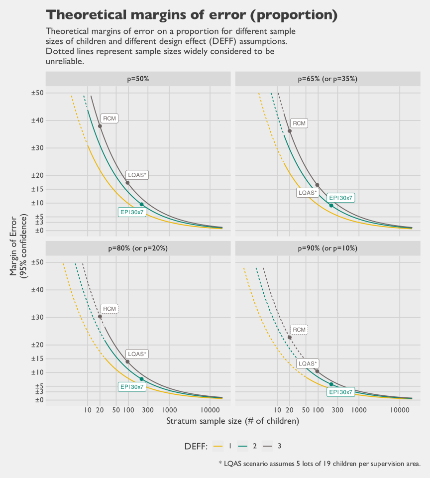
This panel provides a lower-bound planning view under idealized assumptions. The next panel applies the same logic to NSUM, where effective information depends on both respondent count and reported network degree.
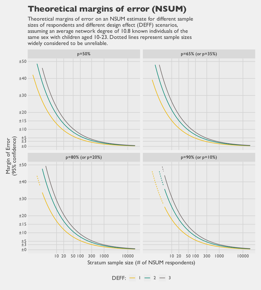
Taken together, the proportion and NSUM curves show the same structural tradeoff. Meaningful gains in precision require rapidly increasing sample sizes once margins of error move into low single digits.
4.3.3.1 Precision Relative to Cost
The theoretical curves above isolate how sampling error scales with sample size. Planning decisions, however, are made in budget space rather than sample-size space. To connect the two, we map theoretical precision to expected cost under two accounting perspectives. The marginal perspective uses direct field implementation cost per additional completed interview. The total perspective uses total financial cost from project expenditure records. This subsection is therefore a financial-cost planning view and does not include non-financial cost components (for example, respondent and stakeholder time valuation). This framing makes diminishing returns explicit and helps distinguish choices that are cost-feasible from those that are only statistically desirable in principle. For this subsection, we narrow the operational precision-cost analysis to the Gold Standard design and parameterize uncertainty with design effects of 1.5, 2, and 3. All other methods are excluded from the precision-cost analysis for method-specific reasons. NSUM and administrative approaches are excluded because the empirical results in this study showed substantial bias. RCM is excluded because it is operationally anchored to a fixed sample size of 20, so sample-size scaling is not decision-relevant. LQAS is excluded because planning is usually based on lot-classification error properties, and pooled prevalence precision additionally requires lot-population structure and representativeness inputs that vary by application. Figure 4.31 and Figure 4.32 then show the precision-cost tradeoff curves under marginal and total financial perspectives. Figure 4.33 shows how much additional precision each increment of spending buys as sample size scales.
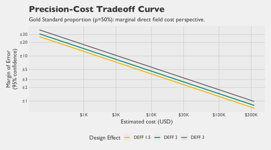
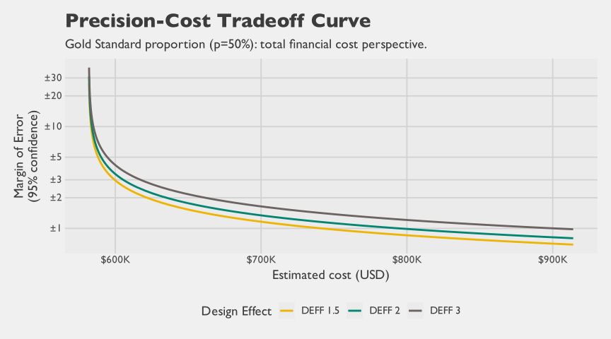
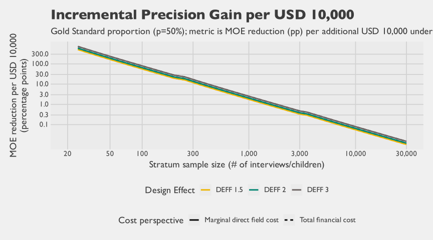
The tradeoff curves in Figure 4.31 and Figure 4.32 show the same qualitative pattern as the sample-size curves, but in more decision-relevant units. Moving from high uncertainty to moderate uncertainty is comparatively inexpensive. Moving from moderate uncertainty to low single-digit margins requires disproportionately larger resources. The incremental-gain curve in Figure 4.33 quantifies that same pattern as an efficiency curve. Early increments in sample size buy relatively large information gains per dollar, while later increments buy progressively less. The log-scaled axes make this curvature easier to see across low- and high-cost ranges in a single view, and the Design Effect (DEFF) curves show the sensitivity of requirements to clustering.
To keep the chapter readable, Table 4.22 presents a compact Gold Standard view under the total financial-cost perspective with DEFF sensitivity, including a ±3% Margin of Error (MOE) target. Expanded Gold Standard tables (including marginal direct-field and total financial perspectives across all thresholds and budgets) are provided in the Technical Details appendix of the full methodological report. Fixed and overhead cost structures can vary substantially across implementing agencies and across funder preferences for quality assurance intensity. The values in Table 4.22 are calibrated to the observed financial cost structure in this study, which was relatively cost-intensive under the Gold Standard implementation model. For scenario planning under alternative assumptions, use the interactive calculator in Appendix B to vary cost structure, marginal cost, and DEFF inputs.
DEFF | Target MOE (95% CI) | Required n | Fixed Financial Cost (USD) | Variable Financial Cost (USD) | Total Financial Cost (USD) | Incremental Total Financial Cost from Previous Threshold (USD) |
|---|---|---|---|---|---|---|
1.5 | 15.0% | 65 | $581,797 | $720 | $582,517 | $310 |
2.0 | 15.0% | 86 | $581,797 | $952 | $582,749 | $410 |
3.0 | 15.0% | 129 | $581,797 | $1,429 | $583,225 | $620 |
1.5 | 10.0% | 145 | $581,797 | $1,606 | $583,403 | $886 |
2.0 | 10.0% | 193 | $581,797 | $2,138 | $583,934 | $1,185 |
3.0 | 10.0% | 289 | $581,797 | $3,201 | $584,997 | $1,772 |
1.5 | 7.5% | 257 | $581,797 | $2,846 | $584,643 | $1,240 |
2.0 | 7.5% | 342 | $581,797 | $3,788 | $585,584 | $1,650 |
3.0 | 7.5% | 513 | $581,797 | $5,682 | $587,478 | $2,481 |
1.5 | 5.0% | 577 | $581,797 | $6,391 | $588,187 | $3,544 |
2.0 | 5.0% | 769 | $581,797 | $8,517 | $590,314 | $4,729 |
3.0 | 5.0% | 1,153 | $581,797 | $12,770 | $594,567 | $7,088 |
1.5 | 3.0% | 1,601 | $581,797 | $17,732 | $599,528 | $11,341 |
2.0 | 3.0% | 2,135 | $581,797 | $23,646 | $605,443 | $15,129 |
3.0 | 3.0% | 3,202 | $581,797 | $35,464 | $617,260 | $22,694 |
These estimates depend on two simplifying assumptions. First, fixed costs are allocated from observed project totals and treated as method-specific constants over the planning range. Second, variable cost is treated as linear in achieved interviews. Both assumptions are useful for transparent planning, but both can shift in new settings where staffing models, logistics, or supervision structures differ.
Taken together, these views show that precision-performance cannot be interpreted without a cost frame. In operational settings, a method may appear attractive by sample-size theory alone but become infeasible once fixed and semi-fixed economic costs are recognized. Conversely, some high-uncertainty designs may still be efficient for screening or supervisory use when decision thresholds are coarse and speed is prioritized.
4.4 Discussion
4.4.1 Time and Cost Drivers
The analysis shows that total cost differences across methods were driven more by scope and fixed effort than by large differences in marginal field effort per interview. Methods with broader implementation footprints and larger setup demands accumulated higher total costs even when per-unit field costs were closer. This pattern is visible in the apportioned phase-by-method breakdown, where preparation, management, and analytical work remain substantial contributors alongside interviewing.
Labor structure also matters as much as labor volume. Field implementation contributes most hours, but specialist analytical and technical roles account for a disproportionate share of financial expenditure. For planning and comparison, this means that reducing interview duration alone cannot fully control budgets if higher-cost analytical phases remain unchanged.
4.4.2 Economic Cost Framing
This chapter estimates economic cost as the sum of financial expenditure and non-financial labor contributions from respondents and stakeholders. That broader framing changes interpretation. A method that appears less expensive in budget terms can still impose substantial unpaid time costs on households and government partners.
Respondent burden is especially important in this setting. Survey participation consumes real time from caregivers who are not paid by the project, so that time has an opportunity cost even when no financial transaction occurs. Including these inputs makes cross-method comparisons more transparent about total resource use from society’s perspective, not only the implementing agency’s accounts.
4.4.3 Exchange Rates
Interpreting costs in USD requires care in a period when the naira-to-dollar exchange rate moved sharply and domestic prices were also rising. Nigeria’s official exchange rate rose from about 426 naira per dollar in 2022 to 645 in 2023 and 1,479 in 2024, implying a large decline in the naira’s USD value over a short period (World Bank 2026b). At the same time, annual Consumer Price Index (CPI) inflation was also elevated, rising from 18.8 percent in 2022 to 24.7 percent in 2023 and 33.2 percent in 2024 (World Bank 2026a). The foreign exchange market reforms initiated in 2023, including window unification and the willing-buyer willing-seller approach, were part of this macroeconomic transition (Central Bank of Nigeria 2025; International Monetary Fund 2024).
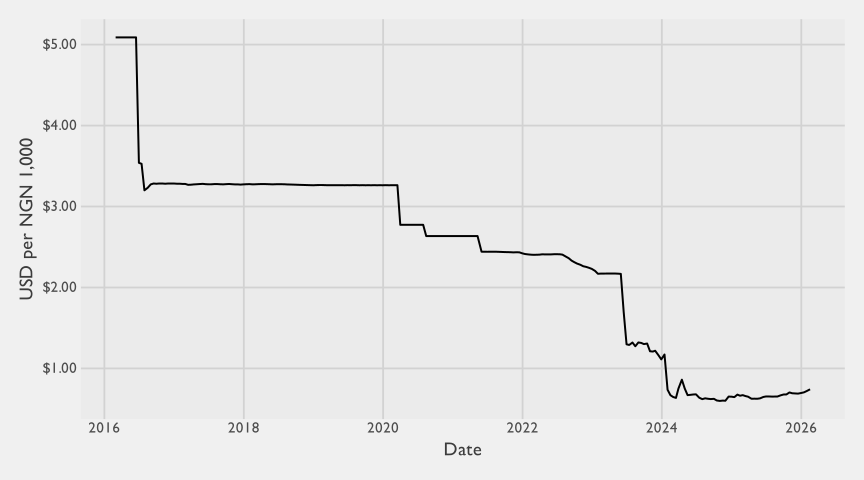
The trend in Figure 4.34 is based on a daily middle-rate series.12
These shifts affect interpretation in two directions. First, for naira-denominated inputs, conversion to USD is highly sensitive to the exchange rate year used. In this report, we use a fixed exchange rate of 0.00074 USD per naira (equivalently, about 1,347 naira per USD). Second, inflation means that naira costs themselves were changing over time, so comparing USD totals across years without deflation or normalization can mix price-level effects with real resource use. The International Monetary Fund (IMF)’s 2024 and 2025 Article IV communications also emphasize this joint movement of exchange-rate adjustment and high inflation in the transition period (International Monetary Fund 2024, 2025).
A simpler way to read magnitudes is to compare exchange-rate levels directly. As shown in Figure 4.34, the shift is not a small year-to-year fluctuation but a large structural change over a short period. In this series, the naira’s USD value a few years ago (around 2022) was roughly three times higher than in 2024–2026 levels. Relative to the mid-2010s, it was roughly six to seven times higher. The same local-currency cost can therefore look about 3x larger in USD under 2022 rates, and about 6–7x larger under mid-2010s rates. For a project like this one, where labor costs span borders and some inputs are paid directly in USD while others are paid in naira, this can materially distort interpretation of relative cost structure. A composition that appears consultant-heavy or internationally expensive under one exchange-rate frame may have looked very different a few years earlier under a different naira-dollar regime.
For planning and budgeting, USD conversion still serves a practical purpose because real project expenditures are often settled in dollars, especially when donor funding is denominated in USD. At the same time, interpretation requires two cautions. First, the external validity of USD-denominated findings depends on exchange-rate stability. For example, if the same observed enumerator time inputs had been valued under 2015 exchange-rate conditions, the USD cost of field data collection alone would have appeared roughly six to seven times larger. Given that enumerator time is a dominant operational input, a roughly six- to seven-fold difference in dollar conversion would materially change the apparent cost structure and the narrative of what drives total cost. Large exchange-rate movements can materially change expected totals and the apparent distribution of financial cost across cost categories. Second, interpretation changes depending on whether burden is expressed as time or as USD. When local respondent or stakeholder time is monetized in naira and converted to dollars, its USD value can appear very small relative to non-Nigerian labor inputs, even when the underlying time burden is substantial. Hours and days are much less sensitive to macroeconomic valuation shifts. Neither lens is complete on its own, so this chapter reports both time burden and USD-valued burden.
4.4.4 Interpretation Limits
Several results in this chapter are descriptive accounting summaries rather than causal estimates. Observed differences across methods combine design choices, implementation scale, and operational context, so they should not be interpreted as pure method effects in isolation.
Respondent opportunity-cost valuation also depends on explicit assumptions. Interview duration is a practical proxy for respondent time, and wealth-based multipliers anchor relative valuation, but these are still approximations. The estimates are most useful for order-of-magnitude comparison and transparency about burden, not for claiming a precise market value of each respondent hour.
Coverage of module-specific metadata also varies across methods. Some diagnostics are cleaner for the core survey streams than for other approaches, which is one reason this chapter occasionally reports core-survey and non-core methods separately.
4.5 Conclusions
Labor is the dominant cost driver, with different implications for time and budget. Field teams account for most person-time, while analysis and technical review account for a large share of financial cost because those activities are concentrated among higher-cost specialists. Cost control therefore depends on both operational efficiency in fieldwork and realistic budgeting for analytical labor.
Total cost differences are driven more by scope and fixed overhead than by marginal field cost. Across methods, marginal field costs per additional unit are more similar than total costs. Large total-cost gaps are driven mainly by implementation scope, sample size, and fixed overhead.
Economic costing changes interpretation by including unpaid time inputs. Non-financial labor from respondents and stakeholders contributes materially to the full resource burden. Interpreting only financial expenditures understates the total social opportunity cost of implementation.
4.6 Recommendations
Plan budgets around labor structure, not only interview counts. Budget models should explicitly separate field labor, analysis labor, and overhead. This makes cost projections more realistic and reduces the risk of under-budgeting technically intensive phases.
Use total and marginal costs together for planning decisions. Total cost is the relevant metric for contracting and implementation choices at a given scale. Marginal cost is the relevant metric for scenario analysis when adding interviews, clusters, or field-days.
Track non-financial inputs as part of routine reporting. Including respondent and stakeholder time in reporting improves transparency about full economic burden and supports more complete comparisons across implementation options.
Broader cross-method recommendations are consolidated in the report conclusion chapter.
An empirical density is a smooth, continuous version of a histogram that helps visualize the overall shape of a distribution. It can be thought of as a smoothed curve drawn over the histogram bars.↩︎
Although heuristic, the 80th percentile usefully bounds duration for four-fifths of cases. Because time distributions tend to be right-skewed, it captures most typical operations without letting a small long tail dominate the summary.↩︎
Unlike Table 4.2, which conditions on a completed child interview, Table 4.5 also includes NSUM-only completions (households with no age-eligible child, which skip the child immunization history module); the Total row median is therefore lower than the “I” row median in Table 4.2.↩︎
For the Gold Standard child module, households were eligible only if a child aged 0–23 months was present. For the NSUM module, households without an age-eligible child could still contribute if an adult respondent was available. In practice, when no eligible child lived at the address, the screener asked whether an adult was available for the NSUM interview.↩︎
The model in question is a multi-level Generalized Additive Model (GAM) with random intercepts for enumerators and fixed effects for the number of age-eligible children interviewed and whether an NSUM respondent was available for interview. A smoothing spline is fit to an index variable that enumerates the temporal order of a given interviewer’s successful survey interviews.↩︎
Although the curve in Figure 4.11 shows a noticeable drop after 300 surveys, this is likely a spurious finding. For one, the uncertainty band in this section is wider. Second, the drop likely reflects that only enumerators who tend to be fastest who end up reaching 300+ interviews. The research team believes that the survivorship bias in the data likely caused the model to overestimate the speed of interviews past the 300th interview.↩︎
Random intercepts represent each enumerator’s deviation from the population-average duration, with estimates shrunk toward zero by an amount that depends on how many surveys the enumerator contributed.↩︎
The model used is a negative binomial GAM with random intercepts for enumerator and LGA effects and smoothing splines on the proportion of LGA sampled cases completed.↩︎
The time and costs of conducting this costing analysis have been netted-out from all totals. They are ancillary to the implementation effort of the methods under comparison and therefore fall outside the costing boundary. No further meta-research activities — methodological simulations, cross-method benchmarking, or chapter-level methodological exposition that went beyond routine operational reporting — have been netted out separately. Some of the largest such activities, most notably the adaptive-sampling simulation work, were conducted after the time-motion data-collection window closed and therefore do not appear in these totals. For meta-research time that does fall within that window, the level of detail at which time was reported is not fine enough to cleanly separate “core” deployment work from methodological exploration. Two further caveats are useful for readers comparing these figures to other implementing arrangements. First, the report devotes a full chapter to each method’s methodology and findings, and likely turns over more stones than a typical operational exercise would for any single method. Second, the labor cost of analysis depends heavily on the staffing mix — heavy involvement of subject-matter experts and consultants (as here) costs substantially more than would a locally hired monitoring-and-evaluation officer. The planning and analysis figures reported in this chapter are therefore best read as upper bounds on what a routine, lean-staffed deployment of each method would have cost in those phases.↩︎
Supervisors were paid $70 United States Dollar (USD) per day and enumerators were paid $18.50 per day. As part of the $70 daily supervisor payment, supervisors were expected to cover the vehicle and fuel costs needed to support their team, even though no explicit split was specified. For this analysis, we treat $18.50 of the $70 as labor costs and attribute the remaining balance to transportation.↩︎
In this pipeline, wealth quintiles are computed from the child-module household frame rather than from all interview streams. As a result, the wealth adjustment is applied primarily to the core child-module interviews (GS and AS, and the subset of NSUM-linked cases with a matched child-module record). For methods/cases without an estimable wealth quintile (for example, all observed RCM cases and most LQAS/NSUM-only cases), the multiplier defaults to 1.0 for unknown cases, so valuation is effectively at the minimum-wage baseline. Re-estimating a harmonized wealth index across all instruments would require additional data engineering and is outside the current pipeline scope.↩︎
The daily series in Figure 4.34 is sourced from Bundesbank’s BBEX3 exchange-rate dataset (via DBnomics), specifically the Nigeria USD middle-rate series (
D.NGN.USD.CA.AC.000).↩︎