Method | Sentinel LGAs | Non-sentinel LGAs |
|---|---|---|
Gold Standard | ✓ | ✓ |
NSUM | ✓ | ✓ |
Adaptive Sampling | ✓ | |
LQAS | ✓ | |
RCM | ✓ | ✓ |
ARR | ✓ | ✓ |
2 Methodology
This report compares a gold-standard multistage cluster probability survey with five alternative approaches for measuring zero-dose prevalence and related vaccination indicators. A direct comparison of headline results is appealing but rarely feasible in any strict sense: the methods were designed for different objectives, operate at different scales, and rely on different units of observation and field footprints. Several components also share fieldwork processes or overlap in sampled units, which affects both inference and cost attribution. This section provides context for interpreting those comparisons: what each method is designed to do, how design choices shape precision requirements, where bias may arise, and how implementation choices and shared logistics affect interpretation. For full details of the baseline survey’s sampling design—including the gridded Enumeration Area (EA) construction, direct building-footprint sampling in the sentinel Local Government Areas (LGAs), and the associated sample size calculations—readers are referred to the Survey Design chapter of the baseline report (Mindset 2025).
2.1 Differing Objectives
If methods were straightforward to compare, they would share a single inferential objective, most naturally population-level prevalence estimation. The methods in this study were built to serve different program decisions, and several balance multiple objectives that compete with one another in design and implementation. Some approaches are optimized for a single aggregate prevalence estimate (for example, Network Scale-Up Method (NSUM)). Others are optimized for classification relative to an operational threshold, with prevalence estimation treated as a secondary output conditional on the decision rule (for example, Lot Quality Assurance Sampling (LQAS)). Many multistage cluster surveys are designed to deliver estimates at multiple levels of aggregation, such as a state estimate alongside LGA-level estimates, which often implies different precision targets across domains and drives larger sample sizes. Some designs are explicitly powered to support inference about change over time (as in the baseline study), while others prioritize rapid identification of zero-dose children for immediate follow-up within selected catchments rather than broad generalization (as in Rapid Convenience Monitoring (RCM)). Because each method was optimized around different objectives and tradeoffs, head-to-head comparisons must account for what each approach was built to do.
The 2025 baseline study used as the benchmark is unusually large by vaccination coverage survey standards. Sample sizes were set so that each of four strata could meet a stratum-specific precision target, and the design was powered to support inference about change in the sentinel LGAs, including detection of relatively small differences at a subsequent assessment.1 These objectives are more demanding than designs focused on a single reasonably precise estimate and therefore increased required sample size relative to conventional Expanded Programme on Immunization (EPI)-style practice. This provides a very precise reference point for judging other methods, but it also means the baseline is not a neutral yardstick for efficiency, because its low error reflects a deliberate design choice driven by planned baseline-to-follow-up comparisons.
2.2 Differing Precision Targets
A head-to-head comparison naturally examines statistical error: how well each method estimates the underlying population quantity, and how much sampling error would be expected under repeated application of the same design in comparable settings. But sampling error is shaped by more than the operational characteristics of a method (such as clustering or stratification) or its field dynamics (such as nonresponse). It also reflects design choices, especially the tolerated error and the sample size and allocation required to achieve it. For this reason, it is not informative to declare a very large gold-standard survey superior simply because it yields lower error than a deliberately small-sample approach such as RCM. A fair comparison asks what each method delivers, in bias and uncertainty, relative to the time, cost, and operational burden it requires, and whether that performance is fit for purpose.
Most methods begin with an explicit or implicit error criterion, framed as a precision bound for an estimate, power to detect change, or a tolerated risk of misclassification. Once specified, it largely determines sample size given the design’s variance structure and expected field conditions. However, methods differ in how much latitude they leave to implementers when setting these targets. Some are highly prescriptive and effectively fix precision through fixed sample sizes or quotas, as in the traditional EPI \(30 \times 7\) design and in RCM protocols that target approximately 20 eligible children per catchment. Other methods are flexible in principle but often converge to common defaults in practice. For example, LQAS can accommodate a wide range of decision risks and sample sizes. In practice, however, many implementations revert to common conventions, such as sampling 19 children per lot. More broadly, classification designs often adopt more permissive Type I error rates, such as \(\alpha = 0.10\). This contrasts with the \(\alpha = 0.05\) convention that is more typical when reporting confidence intervals for prevalence-focused surveys. By contrast, probability-based prevalence designs such as multistage cluster surveys, and indirect estimation approaches such as NSUM, can be implemented across a wide range of precision targets, with sample sizes that vary substantially depending on whether the objective is a single aggregate estimate, disaggregated domain estimates, or inference about change over time. These differing goal posts mean precision comparisons across methods must be interpreted cautiously, because the methods were not designed around a common precision target.
The present study illustrates how strongly these design choices can drive scale. The Gold Standard survey was powered primarily as the baseline against which implementing-partner interventions would be evaluated, and secondarily as a methodological comparator. This required unusually tight precision, and the sample size planning for the Gold Standard stratum samples targeted power to detect a three-point difference in prevalence with 80% power within each sentinel LGA. By comparison, had the study instead followed the widely used EPI benchmark,2 the survey team would have selected 30 clusters with 7 children per cluster for each of the four strata (three Sentinel LGAs and one combined Non-Sentinel area), yielding \(30 \times 7 \times 4 = 840\) children. That scale is far smaller than the roughly twelve thousand interviews ultimately completed in this study.
In other cases, the effective precision targets and resulting sample sizes were driven more by logistical convenience than by a standalone planning exercise. For example, no formal sample size planning was undertaken for NSUM. Because it was implemented as an additional module within the main household questionnaire, its achieved sample size largely inherited the Gold Standard design choices. The realized NSUM sample size also reflected predictable losses driven by the method’s within-household selection step, including nonresponse when the randomly selected adult member was not present.
For LQAS, sample size planning followed common conventions used in other implementations, including The African Field Epidemiology Network (AFENET)’s Decentralized Immunization Monitoring (DIM) approach. In each of the 32 wards across the three Sentinel LGAs, data were gathered on 19 children aged 12–23 months. For RCM, the decision to conduct two RCMs per stratum was pragmatic rather than design-optimal, but the within-location target of approximately 20 eligible children followed RCM guidance.
The latest WHO guidance makes this explicit: sample size should be driven by the study’s inferential objectives and precision targets, not by a single prescriptive template (WHO 2018). Accordingly, the gold standard is best understood as a family of probability-based designs that share core principles and operational practices but vary in scale, domain objectives, and analytic purpose. In this report, the term gold standard refers to these probabilistic foundations and field and analytic practices, and the baseline survey implemented here represents a higher-intensity design than a typical cluster coverage survey.
Given this flexibility in scale, one way to make comparisons more interpretable is to shift from raw precision to a normalized efficiency metric such as the Design Effect (DEFF). When the inferential objective is the same and probability sampling is used, a DEFF can summarize variance inflation relative to a simple random sample of the same nominal size. This provides a measure of design efficiency that can be compared across probability-based approaches even when realized sample sizes differ. However, DEFF has its limits. It is outcome specific and estimand-specific and is not generally meaningful for comparing methods built around different targets, such as classification designs versus prevalence estimation. It also does not address bias: when an estimator is materially biased, DEFF can still describe variance inflation, but it no longer summarizes overall accuracy, which depends on both variance and bias. Because two of the methods assessed showed signs of considerable bias, this further complicated its use as a comparative metric, and we did not prioritize it for that purpose.
2.3 Potential Bias
Precision comparisons are most interpretable when methods can be treated as approximately unbiased for the estimand of interest, but this assumption is not equally plausible across approaches. Some methods introduce clear pathways for bias by design, even when they can be informative in practice. For example, NSUM estimates can be biased by transmission and barrier effects (discussed in the NSUM chapter), and RCM relies on a non-probability walk protocol that may recruit households in a systematically unrepresentative way. Even methods intended to support approximately unbiased inference, such as multistage cluster probability surveys, can exhibit bias in practice due to operational factors such as nonresponse, incomplete screening, or differential contact success across households. Weighting adjustments and strong field procedures can reduce some of these risks, but they cannot guarantee unbiasedness. This complicates head-to-head comparison because bias is often difficult to detect and quantify, and total error reflects both variance and bias that are not easily disentangled. In this report, comparisons are benchmarked to the gold-standard survey for the same population, domain, and reference period where feasible, and large departures by alternative methods are interpreted as consistent with potential bias. The benchmark itself carries uncertainty, however, which limits how decisively such bias can be attributed.
2.4 Implementation Variability
A method label does not uniquely determine either its operational footprint or its inferential properties. Even when two organizations report using the same method, design and field decisions can differ enough to change who enters the sample, how defensible inference is, and what it costs to execute. As a result, nominally identical methods can, in practice, be meaningfully different from one organization to the next.
For some methods, this range reflects built-in flexibility rather than accidental variation, whereas in other cases it reflects that multiple protocols exist under the same umbrella method. For LQAS, results depend on how the classification problem is parameterized, including the lower and upper thresholds, tolerated misclassification risks (for example, \(\alpha\) and the corresponding power), and how the probability sample is operationalized within wards. For RCM, implementation follows World Health Organization (2024) guidance3, but related protocols by similar names exist.4 For example, rapid house-to-house monitoring can incorporate more structured randomization, including multiple random walks, which may change both field burden and inferential interpretability. Furthermore, organizations make distinct operational choices in how the design is carried out. Data collection firms often implement the same nominal design in systematically different ways, reflecting differences in capability, logistics, training, piloting, and quality-control philosophy. Choices about the sampling frame, selection rules, and the discipline with which the selection protocol is followed in the field can materially affect classification performance and interpretability. For multistage probability surveys, implementation quality depends on the stated design and on how clusters and households are actually selected, listed, and screened, and on whether field teams adhere to pre-specified selection rules under operational pressure and temptations. Agencies differ in how strictly they maintain probabilistic selection, whether they substitute convenience or quota approaches when field conditions are difficult, and how aggressively they pursue callbacks and revisits to mitigate nonresponse. These differences affect the error properties of each method and shift both timelines and cost per completed interview.
2.5 Differing Geographic Scope
For practical and comparability reasons, some methods were intentionally limited to specific geographic domains rather than implemented statewide. Table 2.1 summarizes the areas visited by each component.
LQAS was implemented only in the sentinel LGAs, because comparison to the gold standard data would not be possible in non-sentinel areas. The baseline study was not designed or powered to support ward-level (or LGA-level) inference in the non-sentinel stratum, which meant many wards in non-sentinel areas had very little data for comparison. In fact, under the realized random draw, some wards in non-sentinel areas had zero EAs sampled within them in the gold standard sample.
Conversely, the Adaptive Sampling (AS) component was not undertaken in sentinel LGAs. In those areas, sampling fractions were sufficiently high that much of each LGA would have been covered anyway, with interviewed households clustered densely and in close proximity. Because adaptive methods are designed to concentrate marginal sampling effort around detected hotspots, the incremental value of adaptivity was limited under such near-saturation coverage.
Finally, although RCM was not geographically restricted by design, the protocol was implemented as two RCMs locations per stratum (three sentinel LGAs plus one combined non-sentinel stratum). This implies that only two locations would be visited in the non-sentinel stratum, and the random selection resulted in locations in Kiru and Kumbotso.
For head-to-head comparison, these differences in coverage mean that results should be compared within the same geographic domains rather than across unmatched areas.
2.6 Shared Survey Logistics
Several methods in this study were implemented as an integrated field program rather than as fully standalone surveys. As a result, some components shared the same planning, travel, screening, training, supervision, and data-collection infrastructure, and some overlap in sampled units occurred by design or by chance. This matters for two reasons. First, overlap can affect statistical comparisons when the same or related units contribute to multiple estimates, as estimates are not fully independent. Second, it complicates cost efficiency analysis and future planning because observed costs reflect joint production and shared overhead rather than purely method-specific effort.
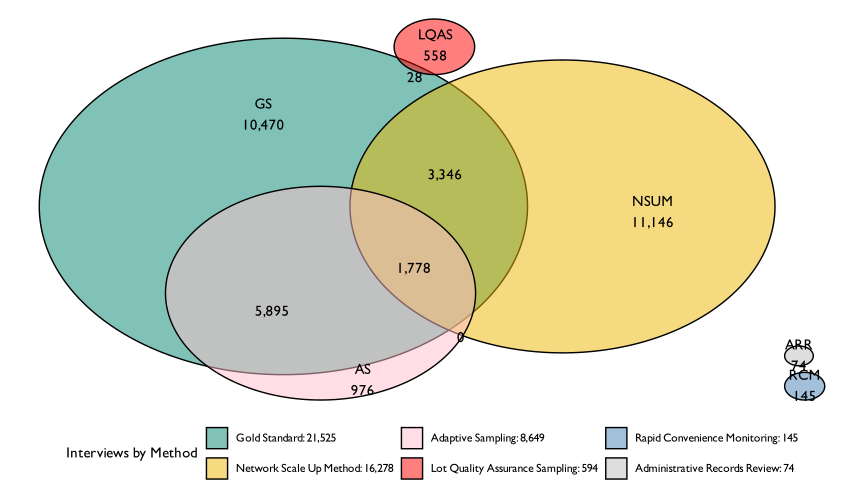
Overlap occurred through three main mechanisms, as shown in Figure 2.1. First, some overlap was structural by design. The adaptive sampling design built on the multistage probability sample by drawing a supplementary sample that was combined with the conventional portion to improve precision. This means the adaptive method necessarily shared upstream sampling and fieldwork processes with the gold-standard survey. Second, some overlap was created for logistical efficiency. The gold-standard household survey included an NSUM module, enabling two approaches to be fielded within the same household-contact and travel footprint, even when the NSUM respondent differed from the primary caregiver respondent. Third, some overlap occurred by chance because sampling fractions were high in some domains. In the sentinel areas, independently drawn LQAS samples occasionally revisited households already interviewed by the gold standard. Where this occurred, previously collected responses were used rather than re-interviewing households with essentially the same instrument.
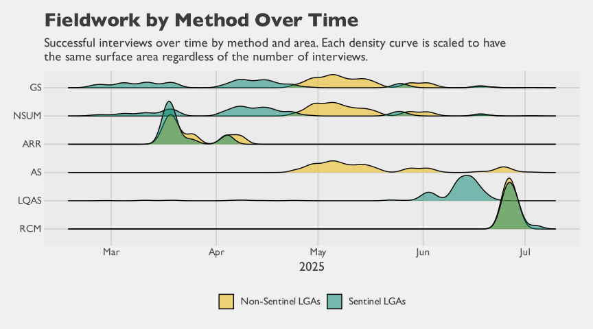
Shared logistics also shaped the timing of data collection. As shown in Figure 2.2, the gold standard, NSUM, and the initial AS component largely coincided because they shared a survey instrument and field teams. In many respects this pooling increased efficiency, but it also created a capacity constraint: the same teams and support staff could only undertake so much at once. As a result, methods that would ideally be fielded concurrently for maximum comparability had to be sequenced. For example, LQAS, RCM, and the AS supplement were implemented later, owing to distinct protocols, separate field plans, and the practical need to stagger workloads.
These shared processes mean that the total observed field costs cannot be interpreted as the standalone cost of each method. They also imply that comparisons based on raw totals can be misleading, because methods differ in both scale and the extent to which they benefited from shared infrastructure. For this reason, the cost analysis later in this report accounts for this joint production process, apportioning shared inputs and overhead as judiciously as possible between methods using a data-driven rule based on each method’s share of successful interviews. Even with careful allocation, shared production limits how directly these cost results generalize to standalone implementations.
Taken together, these comparative challenges motivate the planning tools provided in Appendix B, which allow readers to vary key assumptions, operational parameters, and cost structures, and to see how those choices translate into sample size requirements and expected costs in their own context.
Specifically, the sample was designed to detect a three-point difference in prevalence with 80% power at the level of each Sentinel LGA.↩︎
As noted in the World Health Organization (WHO) reference manual (2018), “[t]here has been a tendency to use a single design (most often 30 clusters of 7 individuals per cluster) without appropriate adaptation of sample size and survey design according to survey goals. The 2005 reference manual (WHO, 2005) gave guidance on how to adapt the design, but in practice this guidance was not often used.” The use of the \(30 \times 7\) benchmark here reflects its ubiquity rather than an implicit pronouncement on its appropriateness for a given set of survey objectives. Indeed, the maximal \(\pm 10\) percentage-point Margin of Error (MOE) that this design induces may often be unacceptably imprecise for many applications.↩︎
The version used for this study’s RCM implementation was an earlier version of this guidance branded by United States Agency for International Development (USAID)/MOMENTUM (MOMENTUM 2024). The core implementation features are substantially the same between the two versions; the newer WHO debranded version includes additional resources and a toolkit for conducting root-cause analysis.↩︎
The acronym RCM is also sometimes used for rapid coverage monitoring, an entirely distinct family of methods unrelated to the rapid convenience monitoring approach evaluated here. We use RCM throughout this report to refer exclusively to the latter.↩︎