Appendix E — PPS sampling with outdated enumeration frames
Probability Proportional-to-Size (PPS) sampling of enumeration areas is one of the most common first-stage designs in household surveys. Under PPS, each candidate Enumeration Area (EA) is drawn with a probability proportional to a Measure of Size (MOS) — typically the EA’s household or population count in the sampling frame. Coupled with a (near-)fixed second-stage take per selected EA, PPS yields roughly equal inclusion probabilities for households across the population, which is why it is the workhorse first stage for national household surveys, DHS-style multi-stage designs, and Multiple Indicator Cluster Survey (MICS). Even methods that are sometimes framed as less rigorous than a World Health Organization (WHO) cluster coverage survey can be set up as genuine probability samples with an EA stage one. The implementation of Lot Quality Assurance Sampling (LQAS) used in this study, based on the Decentralized Immunization Monitoring (DIM) approach, is one such case: stage one draws EAs via PPS from a frame of Government Enumeration Areas (GEAs), and stage two draws households within each selected EA.
EAs themselves come from one of two sources. The de novo path is to build gridded EAs over a population surface — this is what GRID3 and related efforts produce. The more traditional path is to ask the national statistical agency to draw a sample from their frame of EAs, which is typically created or updated during a census year. Either way, the frame has a vintage, and that vintage eventually diverges from current reality as populations grow, shift, and urbanise.
The concern this annex explores is what happens when the frame’s MOS is out of date relative to the population being surveyed today. A pithy version of the answer: stale measures of size produce surveys that are still approximately unbiased on average, but less precise per survey — the confidence intervals widen as the MOS drifts further from reality, even though the point estimates remain centred on the right value over many hypothetical repeats of the design. The bias-vs-efficiency distinction matters because efficiency loss is quiet: a survey with a stale frame does not announce itself with systematically wrong numbers; it announces itself with intervals that are wider than they would be under a fresh frame, which readers often do not notice or attribute to frame age.
Listing, bias, and weights
The “approximately unbiased” claim above carries one methodological footnote worth making explicit. Unbiasedness of a PPS estimator depends on knowing the correct inclusion probability at each stage. Under a fully specified probability design, every selected EA is first listed (or screened): enumerators visit the EA and enumerate every household in it, so that the second-stage sampling probability used at estimation time is the correct one for that EA’s current household count — not the frame’s cached count. Fresh listing decouples stage-two weights from frame vintage: even if the first-stage MOS is out of date, the stage-two correction absorbs the drift.
Full-scale multi-stage cluster surveys — for example, the DHS, MICS, and WHO-style vaccination coverage cluster surveys — typically do perform a fresh listing of each selected EA before household selection, for exactly this reason. Lighter-weight methods designed to be cheaper or faster to field — including our implementation of LQAS, which follows the DIM approach — often skip the listing step and derive stage-two sampling probabilities from the frame’s own household count. In those cases, the weights inherit whatever error the frame carries at that EA. The practical consequences split by estimand:
- For a population mean (which is what “coverage” is — the proportion of eligible children who received a dose), the drift enters through the relative weights across EAs. Relative weights still yield approximately unbiased point estimates provided the drift is uninformative, i.e. uncorrelated with the outcome. If drift is informative — if EAs whose MOS is most out of date are also EAs where the outcome is systematically different — the mean acquires a bias whose sign tracks the drift.
- For a population total (e.g., absolute number of zero-dose children in a jurisdiction), the absolute scaling of the weights matters directly and a stale MOS propagates to the total.
What remains true in both cases is that stale stage-two weights are always noisier than listing-derived weights, and noisier weights mean wider design-based confidence intervals. That is the efficiency loss the rest of this annex is concerned with.
The Nigerian frame
Nigeria’s last census was in 2006. The National Population Commission (NPC) and the National Bureau of Statistics publish post-censal population estimates, but the methodology for updating to current figures is not accompanied by published accuracy measures, so it is difficult for a secondary user to place a quantitative bound on how much any given EA’s MOS may have drifted. For the LQAS sample used in this study, the PPS draw was carried out against the NPC frame. What we received from NPC in return was a list of sampled GEAs together with a relative MOS index per EA — a rescaled share, not absolute household or population counts. That is consistent with the custodial caution statistical agencies sensibly apply to frame-level data that is itself being continuously re-estimated. For our purposes it means the practical question is not “is the absolute MOS correct?” (we never saw absolute MOS values) but rather “do the relative shares across EAs still reflect 2025 reality?”. As with every multi-year-old frame, the answer is almost certainly “not exactly”. The remainder of this annex tries to put a shape on the drift using the Global Human Settlement Layer (GHSL) Degree-of-Urbanization layer as a proxy for how the underlying population has changed.
Figure E.1 juxtaposes the two epochs of the GHSL Degree-of-Urbanization raster over Kano to make the drift concrete. Dragging the vertical handle from left to right reveals 2025 in place of 2005: what reads as a large swathe of Mostly uninhabited area (collapsed into our Village label — see the Class collapse caveats section below) outside the Kano urban core in 2005 has filled in substantially with Suburban / peri-urban classification by 2025. The urban core itself, classified City in both epochs, is essentially unchanged; the growth and reclassification happens on its periphery. A frame whose MOS is anchored to the 2005 (or earlier 2006-census) population surface will therefore assign relative sampling weight to EAs based on their pre-growth configuration, even where the EA itself has since moved up the urbanisation gradient.
A “sample point” in what follows is the Global Positioning System (GPS) coordinate of the household that was actually interviewed for LQAS in a given GEA, not a GEA-level summary. Because the LQAS design tests one eligible child per GEA-lot, there is at most one interviewed-household point per GEA, and the Global Human Settlement Layer Settlement Model (SMOD) class is extracted at that point. This matters where a GEA straddles a boundary between classes (large or elongated GEAs on the urban fringe can contain both Village and Suburban cells, for instance); a GEA-level aggregation would have to pick a modal or centroid class in those cases, whereas an extraction at the interviewed point directly reflects what the enumerator was standing on.
Of the 608 GEAs sampled at stage one, 594 have an interview-point GPS coordinate (the LQAS fieldwork reached an eligible child there); the remaining 14 dropped out of dsg_lqas upstream for fieldwork reasons unrelated to SMOD (no eligible child located, security redirects, or similar). Rather than discard those 14 GEAs from the urbanisation diagnostic, we fall back to the GEA polygon centroid from the LQAS stage-one shapefile and extract the SMOD class there. The descriptive cross-tabulation below therefore reports all 608 stage-one GEAs. The design-based Generalized Linear Model (GLM) further on still runs only on the 594 interview-point rows, because the 14 centroid fallbacks have no child-level outcome or survey weight attached.
Class collapse caveats
The raw GHSL SMOD layer distinguishes eight cell classes. Throughout this report we collapse those eight into four (Table E.1) to keep factor levels stable when cross-tabulating or regressing on urbanisation: several of the raw classes are very sparsely populated in our study area, and left un-collapsed they produce empty or near-empty ward × class cells that destabilise calibration weights. The collapse is therefore driven by statistical tractability, not by geographic correspondence. A consequence is that two of the four labels we use here are deliberate oversimplifications rather than literal descriptions of what is on the ground:
- Village is a catch-all that groups the genuine rural-cluster class (GHSL 13) with a Dispersed rural area class (12), a Mostly uninhabited area class (11), and Water body cells (10). A cell labelled “Village” in the analysis below is therefore not guaranteed to contain a settled village; it only guarantees that the cell is below the suburban density threshold.
- Town groups Semi-dense town (22) with Dense town (23) under a single label.
The Suburban and City labels map one-to-one onto their raw GHSL classes (21 and 30 respectively) and can be read at face value. When we speak of urbanisation transitions in the rest of this annex, those transitions are transitions on the four-level collapsed scale, not on the raw eight-level SMOD scale.
Collapsed label | Raw GHSL code | Raw GHSL class name |
|---|---|---|
Village | 13 | Village (rural cluster) |
12 | Dispersed rural area | |
11 | Mostly uninhabited area | |
10 | Water body | |
Suburban | 21 | Suburban or peri-urban area |
Town | 22 | Semi-dense town |
23 | Dense town | |
City | 30 | City |
SMOD drift, 2005 to 2025
Table E.2 cross-tabulates the GHSL Degree-of-Urbanization class at each sampled GEA between the 2005 epoch and the 2025 epoch. Of 608 GEAs with classifications at both epochs, 172 (28%) fall in a different class in 2025 than they did in 2005. Class reclassification is one-directional: no GEA moves down the urbanization gradient.
The MOS-staleness signal is carried almost entirely by Gabasawa and Gaya. Nassarawa contributes nothing: all 209 of its sampled GEAs sit in the dense urban core (GHSL class City) at both 2005 and 2025, so the MOS-staleness mechanism is structurally absent there and the weighting-drift argument does not apply. Readers should therefore treat Nassarawa as a baseline-coverage comparator in the cross-tabulation below rather than as evidence for or against staleness.
2025 class | ||||||
|---|---|---|---|---|---|---|
Village | Suburban | Town | City | Total | ||
2005 class | Village | 52 | 118 | 31 | 0 | 201 |
Suburban | 0 | 70 | 23 | 0 | 93 | |
Town | 0 | 0 | 68 | 0 | 68 | |
City | 0 | 0 | 0 | 246 | 246 | |
Total | 52 | 188 | 122 | 246 | 608 | |
Figure E.3 visualises the same transitions as the cross-tabulation above, but in a flow form. Ribbons are coloured by 2005 source class and drawn translucent when the class is unchanged (stable) and more opaque when the GEA is reclassified — which makes the upward-only pattern and the volumes involved immediately legible. The By sentinel Local Government Area (LGA) tab breaks the same data apart by fieldwork LGA, so that Gabasawa’s pronounced Village-to-Suburban fan, Gaya’s mixed reshuffle, and Nassarawa’s complete stasis read off the page separately.
Under the same-child population served by the same stage-one sampling frame, a point now classified as Suburban that was rural in 2005 illustrates the MOS-staleness mechanism directly: its current share of the ward’s eligible children is not what the 2006 census assumed, so weights built on the original frame drift from the weights that current population shares would imply.
Zero-dose by urbanisation
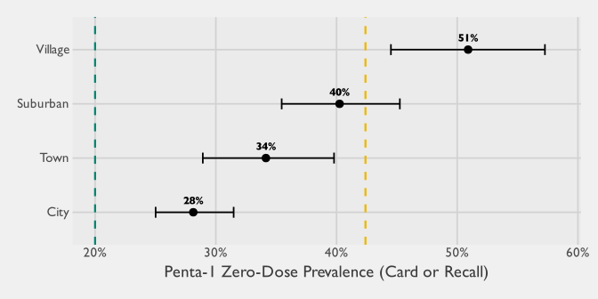
The urbanisation drift documented above would be a curiosity, not a concern, if Penta-1 zero-dose prevalence were uncorrelated with where on the urbanisation gradient a GEA sits. It is not. Figure E.4 reproduces the GHSL Degree-of-Urbanization stratum from the gold-standard household-survey estimates reported in the Kano zero-dose baseline study (Mindset 2025) (findings-132-ri-coverage-zero-dose). Zero-dose prevalence is markedly lower in the dense urban core (City) and rises monotonically across Town, Suburban, and Village cells. The gap between the City point estimate and the Village point estimate is large relative to the Confidence Interval (CI) on either, so the gradient is not an artefact of within-stratum noise.
As an exploratory probe into whether the MOS-drift mechanism is visible at the point-estimate level, we can further stratify the gold-standard estimates by whether each interviewed child’s GEA kept its SMOD class between 2005 and 2025 (stable) or moved up the urbanisation gradient (reclassified). The 2005 and 2025 classes are extracted at the child’s GPS coordinate in exactly the way the LQAS stratification was done above, just applied to the gold-standard household survey. We restrict this analysis to the three sentinel LGAs (Gabasawa, Gaya, Nassarawa) rather than to Kano-wide data so the scope aligns with the LQAS-sampled area that the rest of this annex concerns itself with; a broader sensitivity on all 15 LGAs tells a different (and less coherent) story, mostly driven by a handful of peripheral LGAs outside the LQAS catchment that have urbanised into the City class since 2005. Under the hypothesis that a GEA’s current catchment profile carries residual signal from its pre-urbanisation configuration — the inside-the-sample expression of MOS-drift — reclassified GEAs should carry systematically higher Zero-Dose (ZD) prevalence than stable GEAs of the same 2025 class. Village has no reclassified members by construction (it is the lowest class) and, in the sentinel LGAs, City reclassification is effectively absent (only 4 children sit in GEAs that moved into City since 2005 — Nassarawa was already overwhelmingly City in 2005). The comparison is therefore meaningful for Suburban and Town. Figure E.5 shows the stratification.
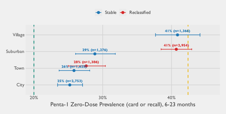
Within the sentinel LGAs, the stratified picture is clean and directionally consistent with the MOS-drift hypothesis. At Suburban, reclassified GEAs (almost all urbanised from Village since 2005) carry notably higher ZD than stable Suburban GEAs — roughly 41% vs 29%, with non-overlapping intervals. At Town, reclassified and stable GEAs sit close together (28% vs 26%, overlapping intervals): once a cell has already urbanised past Suburban, whether it did so in the last two decades or before 2005 no longer predicts a meaningful ZD differential.
The two design-based Wald tests back up this reading. A pooled test of the reclass main effect in an additive GLM (zd_cp1 ~ smod_2025 + reclass) is strongly significant: F = 27.99 (1, 495 df), p = <0.001. Allowing the reclass effect to vary by 2025 SMOD class (zd_cp1 ~ smod_2025 * reclass, fit on the Suburban / Town subset where the interaction is identifiable in the sentinel sample) is also significant: F = 6.30 (2, 494 df), p = 0.002. The interaction reflects the Suburban-vs-Town difference in the reclassified-vs-stable gap — the reclassified-vs-stable log-odds contrast is +0.53 at Suburban and attenuates by about -0.43 at Town, consistent with the picture the figure shows.
That the signal concentrates at Suburban is exactly where the MOS-drift mechanism predicts it should. Gabasawa and Gaya — the two sentinel LGAs that actually have Village-to-Suburban reclassification since 2005 (see Figure E.2) — are the peri-urban fringe of metropolitan Kano, and their newly-Suburban GEAs are precisely the cells whose 2006-era MOS under-represents current population relative to what a fresh listing would show. The observation that those cells also carry higher ZD than already-Suburban cells of similar 2025 classification is exactly the “informative drift” case flagged in the Listing, bias, and weights section: it suggests that, in addition to the always-present efficiency loss, there is a small directionally-consistent bias — the LQAS design under-samples children from the demographic profile that is most likely to be ZD. The size of the contrast (~12 percentage points within Suburban) is large enough that the annex’s overall “approximately unbiased, just less precise” headline deserves the caveat that the approximation is weakest exactly where the GEAs have urbanised the most. A more striking way to see the same result is to notice that the reclassified-Suburban point estimate (41%) sits essentially on top of the stable-Village estimate (41%) — and roughly 12 percentage points above the stable-Suburban estimate (29%). In other words: on the ZD outcome, peri-urban GEAs that urbanised since 2005 behave as though they were still Village, not as though they were Suburban.
Several candidate mechanisms are consistent with that pattern, and the data here cannot adjudicate between them. The most direct is a supply-side story: health-facility coverage, routine-immunisation outreach, and campaign logistics all follow built settlement, and they tend to follow with a lag of years rather than months — the buildings arrive, the services arrive eventually. A more specific version of that story, which we find compelling but speculative, is that the targeting infrastructure used by routine outreach and campaign partners (settlement rosters, facility catchment lists, LGA micro-plans) is typically built against the same vintage of population data that feeds the sampling frame: newly-urbanised peri-urban cells that were sparsely populated at the 2006 census may simply not appear in the settlement rosters that determine where teams go, even if the households are now numerous enough for a satellite-derived SMOD layer to label the cell Suburban. Under that reading, the MOS-staleness phenomenon this annex quantifies at the sampling layer is the visible half of a wider pattern of administrative data lag: the planning layer that shapes service delivery drifts from reality on roughly the same timeline, for roughly the same reason, and at roughly the same cells, which would explain why our newly-Suburban sample behaves in vaccination terms as though it were still Village. Two further mechanisms are also consistent with the pattern: migrant composition (peri-urban fringes draw rural-origin households whose care-seeking behaviour reflects their place of origin more than their place of residence) and SMOD measurement noise at 1 km resolution (a cell reclassified Suburban on satellite may in fact remain functionally Village on the ground). None of these can be ruled in or out from the data we have.
Two cautions are worth emphasising before drawing conclusions from the stratified analysis. First, the sentinel-LGA restriction was not incidental: in a Kano-wide sensitivity (see the commentary above), the City stratum rather than Suburban carries most of the signal, driven by a handful of peripheral LGAs outside the LQAS catchment where new urban classification is appearing for the first time. The GEA-level pattern is therefore clearly LGA-specific, and the “reclassified cells behave like their old class” statement should not be read as a claim about Nigeria or even Kano as a whole. Second, with only three sentinel LGAs the stratification of the interaction model rests on a single LGA-pair (Gabasawa and Gaya) contributing the reclassified-Suburban signal; a fourth sentinel LGA with a different urbanisation trajectory could pull the direction differently. The defensible take-away is narrower than the point estimates suggest: there are clear geospatial structural effects on ZD prevalence that operate at a finer scale than the SMOD class label captures, and those effects are worth exploring further even if the current data are not powered to generalise them.
The relevance to this annex is direct. The outcome of the study is correlated with the dimension on which the frame has drifted. That satisfies the condition under which stale-MOS efficiency loss — and, in the unfavourable case where the drift is also informative, a small residual bias — can bite on estimates of ZD prevalence. In principle, a GEA whose effective 2025 urbanisation profile differs from what the frame’s MOS implies is exactly the kind of unit that will carry more variance than the design budgeted for.
Readers seeking a headline should take away two things: first, the study’s estimates remain approximately unbiased under the conditions discussed in Listing, bias, and weights; second, the confidence intervals around those estimates are almost certainly wider than they would be under a freshly-listed 2025 frame, and that widening falls disproportionately on the GEAs that have urbanised the most since 2005 — which Figure E.4 and Figure E.5 together suggest are also the GEAs where zero-dose prevalence is highest.